The Aggregate Expenditures Model
17. The Aggregate Expenditures Model. 17.1. Chapter Objectives. Economists Combine Consumption and Investment to Depict an Aggregate Expenditures Schedule for a Private Closed Economy Three Characteristics of the Equilibrium Level of Real GDP in a Private Closed Economy AE = Output

The Aggregate Expenditures Model
E N D
Presentation Transcript
17 The Aggregate Expenditures Model 17.1
Chapter Objectives • Economists Combine Consumption and Investment to Depict an Aggregate Expenditures Schedule for a Private Closed Economy • Three Characteristics of the Equilibrium Level of Real GDP in a Private Closed Economy • AE = Output • Saving = Investment • No Unplanned Changes in Inventories • How Changes in Equilibrium Real GDP Occur and Relate to Multiplier • Integrate Public sector and Foreign Sectors into AE • Recessionary and Expansionary Expenditure Gaps
Consumption and Investment • Simplifications • Private Closed Economy • Planned Investment • Investment Schedule Investment Demand Curve Investment Schedule Investment Demand Curve Investment Schedule Ig 20 Investment (billions of rand) rand i (percent) 8 20 20 ID 20 Investment (billions of rand) Real GDP (billions of rand)
Consumption and Investment • Equilibrium GDP: C + I = GDP Y = C + I Y = Co +cYd + I • Real Domestic Output (Yd) • Aggregate Expenditures (Y) • Aggregate Expenditures Schedule • Equilibrium GDP • Disequilibrium 17.1
(5) Investment (I) (6) Aggregate Expenditures (C+I) (7) Unplanned Changes in Inventories (+ or -) (1) Real Domestic Output (and Income) (GDP=Yd) (4) Saving (S) (1-2) (2) Con- sump- tion (C) (8) MPC Consumption and Investment (3 (Co) …in Billions of rand R370 390 410 430 450 480 490 510 530 550 R377.5 392.5 407.5 422.5 437.5 460.0 467.5 482.5 497.5 512.5 R100 100 100 100 100 100 100 100 100 100 R-7.5 -2.5 2.5 7.5 12.5 20 22.5 27.5 32.5 37.5 20 20 20 20 20 20 20 20 20 20 R397.5 412.5 427.5 442.5 457.5 480 487.5 502.5 517.5 532.5 R-27.5 -22.5 -17.5 -12.5 -7.5 0 +2.5 +7.5 +12.5 +17.5 0.75 0.75 0.75 0.75 0.75 0.75 0.75 0.75 0.75 0.75 Graphically…
Consumption and Investment • Mathematical Calculations
530 510 490 480 450 430 410 390 370 Consumption (billions of rand) 45° 388 400 420 440 460 480 500 520 540 560 Disposable Income (billions of rand) Consumption and Investment Equilibrium GDP C + I C + I = GDP) C Equilibrium Point Aggregate Expenditures I= R20 Billion C = R460 Billion 17.1
Equilibrium GDP • Other Features… • Saving Equals Planned Investment • Leakage • Injection • No Unplanned Changes in Inventories
Savings and Investment • Mathematical Calculations
510 490 470 450 Aggregate Expenditures (billions of rand) 45° 440 460 480 500 520 Real GDP (billions of rand) Changes in Equilibrium GDP …and the Multiplier (C + Ig)1 (C + Ig)0 (C + Ig)2 Increase in Investment Decrease in Investment
Adding the Public Sector C + Ig + G = GDP • Leakages • Injections • No Planned Inventory Changes S + T = Ig + G 17.2 17.2
(5) Investment (I) (6) Exogenous Public sector Spending (G) (7) Aggregate Expenditure (C+I+G) (1) Real Domestic Output (and Income) (GDP=Yd) (4) Saving (S) (1-2) (2) Con- sump- tion (C) Adding the Public Sector Public sector Purchases and GDP (3 (Co) …in Billions of rand 20 20 20 20 20 20 20 20 20 20 20 R417.5 432.5 447.5 462.5 477.5 500 507.5 522.5 537.5 552.5 560 20 20 20 20 20 20 20 20 20 20 20 R370 390 410 430 450 480 490 510 530 550 560 R377.5 392.5 407.5 422.5 437.5 460.0 467.5 482.5 497.5 512.5 520 R100 100 100 100 100 100 100 100 100 100 100 R-7.5 -2.5 2.5 7.5 12.5 20 22.5 27.5 32.5 37.5 40 Graphically…
Aggregate Expenditures (billions of rand) 45° 470 550 Real GDP (billions of rand) Adding the Public Sector Public sector Spending and GDP C + I + G C + I C Public sector Spending of R20 Billion R20 Billion Increase in Public sector Spending Yields an R80 Billion Increase In GDP
Adding the Public sector • Mathematical Calculations
Adding the Public sector (S=I+G) • Mathematical Calculations
Adding G and the Multiplier • Mathematical Calculations lllllllllllllllllllllllllllllllllllllllllllllllllllllllllllllllllllllllllllllllllllllll
llllllllllllllllllllllllllllllllllllllllllllllllllllllllllllllllllllllllllllllllllllllllllllllllllllllllllllllllllllllllllllllllllllllllllllllllllllllllllllllllllllllllllllllllllllllllllllllllllllllllllllllllllllllllllllllllllllllllllllllllllllllllllllllllllllllllllllllllllllllllllllllllllllllllllllllllllllllllllllllllllllllllllllllllllllllllllllllllllllllllllllllllllllllllllllllllllllllllllllllllllllllllllllllllllllllllllllllllllllllllllllllllllllllllllllllllllllllllllllllllllllllllllllllllllllllllllllllllllllllllllllllllllllllllllllllllllllllllllllllllllllllllllllllllllllllllllllllllllllllllllllllllllllllllllllllllllllllllllllllllllllllllllllllllllllllllllllllllllllllllllllllllllllllllllllllllllllllllllllllllllllllllllllllllllllllllllllllllllllllllllllllllllllllllllllllllllllllllllllllllllllllllllllllllllllllllllllllllllllllllllllllllllllllllllllllllllllll Adding G and the Multiplier • Mathematical Calculations
(6) Investment (I) (7) Exogenous Public sector Spending (G) (8) Aggregate Expenditure (C+I+G) (1) Real Domestic Output (and Income) (GDP=Yd) (3) Con- sump- tion (C) (5) Saving (S) Adding the Public Sector Public sector Taxes and the GDP (2) Taxes (T) (4) (Co) …in Billions of rand 20 20 20 20 20 20 20 20 20 20 20 20 R402.5 417.5 432.5 447.5 462.5 485.0 492.5 500 507.5 522.5 537.5 545.0 20 20 20 20 20 20 20 20 20 20 20 20 R370 390 410 430 450 480 490 500 510 530 550 560 R362.5 377.5 392.5 407.5 422.5 445.0 452.5 460 467.5 482.5 497.5 505 R100 100 100 100 100 100 100 100 100 100 100 100 R-12.5 -7.5 -2.5 2.5 7.5 15.0 17.5 20 22.5 27.5 32.5 35.0 20 20 20 20 20 20 20 20 20 20 20 20 Graphically…
Aggregate Expenditures (billions of rand) 45° 500 560 Real GDP (billions of rand) Adding the Public Sector Lump-Sum Tax Increase and GDP C + I + G C + I + G (with T) R15 Billion Decrease In Consumption From a R20 Billion (MPC=.75) Increase in Taxes R20 Billion Increase in Taxes Yields a R60 Billion Decrease In GDP
Adding the Public sector • Mathematical Calculations
Adding the Public sector (S+T=I+G) • Mathematical Calculations
Adding T and the Multiplier • Mathematical Calculations
540 520 500 480 460 Aggregate Expenditures (billions of rand) 45° 460 480 500 520 540 Real GDP (billions of rand) +5 0 -5 Net Exports Xn (billions of rand) Real GDP International Trade Net Exports and Equilibrium GDP C + I +G +Xn1 C + I +G Aggregate Expenditures with Positive Net Exports C + I + G +Xn2 Aggregate Expenditures with Negative Net Exports Positive Net Exports Xn1 480 500 520 Xn2 Negative Net Exports
International Trade • Net Exports and Aggregate Expenditures • Net Exports Schedule • Net Exports and Equilibrium GDP • Positive Net Exports • Negative Net Exports
GLOBAL PERSPECTIVE -700 200 150 100 50 0 50 100 150 200 250 International Trade Net Exports of Goods - Select Nations, 2004 Negative Net Exports Positive Net Exports +37 Canada -17 France Germany +195 -2 Italy Japan +111 -117 United Kingdom -707 United States Source: World Trade Organization
550 530 510 490 470 Aggregate Expenditures (billions of rand) 45° 490 510 530 Real GDP (billions of rand) Equilibrium Versus Full-Employment GDP Recessionary Expenditure Gap AE0 R5 Billion Gap Yields R20 Billion GDP Change AE1 Recessionary Expenditure Gap = R5 Billion Full Employment
550 530 510 490 470 Aggregate Expenditures (billions of rand) 45° 490 510 530 Real GDP (billions of rand) Equilibrium Versus Full-Employment GDP Inflationary Expenditure Gap AE2 AE0 Inflationary Expenditure Gap = R5 Billion R5 Billion Gap Yields R20 Billion GDP Change Full Employment
Equilibrium Versus Full-Employment GDP • Limitations of the Model • Does Not Show Price Level Changes • Ignores Premature Demand-Pull Inflation • Limits Real GDP to the Full-Employment Level of Output • Does Not Deal with Cost-Push Inflation • Does Not Allow for “Self-Correction”
Say’s Law - The Great Depression and Keynes Last Word • Classical School – Automatic Self-Adjustment to Full Employment – Mill, Ricardo • Views Based Upon “Say’s Law” - J.B. Say (1767-1832) – Supply Creates its Own Demand • Great Depression Caused Questions • Keynes Answered in his General Theory of Employment, Interest, and Money • Income and Saving Discrepancies • Volatility in Investment Spending • Cyclical Unemployment Can Occur • Public sector Should Be Active in the Recovery Process 17.2
planned investment investment schedule aggregate expenditures schedule equilibrium GDP leakage injection unplanned changes in inventories lump-sum tax net exports recessionary-expenditure gap inflationary-expenditure gap Key Terms
Next Chapter Preview… Aggregate Demand and Aggregate Supply Chapter 18!