Understanding Aggregate Expenditures and Demand: A Student Guide to Macroeconomic Concepts
This guide provides a comprehensive overview of aggregate demand (AD) and aggregate expenditures (AE), vital components in understanding macroeconomic principles. It covers the relationship between planned spending, consumption, savings, and investment, explaining concepts like marginal propensity to consume (MPC) and the simple multiplier effect. By analyzing how economic agents plan their spending at various income levels, students will gain insights into the factors affecting economic equilibrium, the role of government spending and taxes, and the implications of injections and leakages in the circular flow of income.

Understanding Aggregate Expenditures and Demand: A Student Guide to Macroeconomic Concepts
E N D
Presentation Transcript
AGGREGATE EXPENDITURES Frederick University 2014
Aggregate Demand (AD) AD – the quantity of GDP, which the economic agents are planning to buy at every price level,ceteris paribus (Y = const)
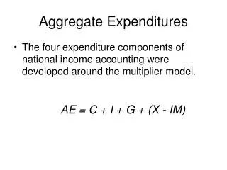
Aggregate Expenditures • АЕ – the expenditures that economic decision makers are planning to make at every level of income, ceteris paribus • Planned Spending • Real GDP = NominalGDP • AE = C + I + G + X - M
Consumption Spending (С) • С – the expenditures that households are planning to make at every level of income, ceteris paribus
Consumption Spending (С) • 500 – consumption spending which does not depend on income, autonomous consumption – С0(Ca, a)
Consumption Spending (С) • C = C0 + (Δ C /ΔY) x Y • Δ C /ΔY – the increase in consumption spending, caused by the increase in income – marginal propensity to consume – MPC (mpc, b) • C = C0 + MPC x Y
Consumption Spending (С) • C = C0 + MPC x Y • MPC = ¾ = 0,75 • If income rises by$100,households increase their consumption spending by $75 and increase their savings by $25 • If income rises by $500, С risesby 5 х $75 = $375 • C = 500 + 375 = 500 + 0.75 x 500
Savings(S) • Marginal propensity to save – the increase in savings, caused by the increase in income: • MPS = Δ S /ΔY • If income rises by$100, and households raise their consumption spending by $75, savings increase by$25 • MPC + MPS = 1 • C + S = Y • S = Y – C = Y – (C0 + MPC x Y) = Y - C0 - MPC x Y = - C0 + Y - MPC x Y = - C0 + Y(1 - MPC) • S = - C0 + MPS x Y
Consumption Spending (С) and Savings (S) • Y = 1000 • C = 500 + 0.75 x 1000
Consumption Spending (С) D 2000 C C = 500 + 0.75Y B 875 375 500 A 500 450 0 Y 2000 500
Factors determining C • Households’ income • Indirect taxation • Propensity to buy imported goods and services • Direct taxation • Consumers’ expectations • Availability of consumer credit • Income distribution • Living standards • Efficiency of market institutions
Investment spending I = Gross Private Domestic Investment • I – Depreciation = Net Investment • Net investment = Purchases of New Equipment + Change in Inventories • Fixed Investment = Depreciation + Purchases of New Equipment • Net Fixed Investment = Purchases of New Equipment • Inventories = • Raw Material • + Unfinished Production • + Finished Goods
Factors determining Investment Spending (I) • Interest rate (i) • Expected future profits (π) • Risk • Excess capacity • Capital-output ratio (α) • Technological changes • Cost of production • Competitiveness of markets • Depreciation policies • Efficiency of market institutions
AE D 2000 C AE = C + I + G + X - M C B 875 375 500 A 500 450 0 Y 2000 500
Leakages imports М Injections exports Х Government purchases G taxes Т Expenditures on final goods and services AE Investment І Final goods and services savings S Macroeconomic Equilibrium I + G + X = S + T + M (I - S) = (T - G) + (M - X) HOUSEHOLDS FIRMS Production factors Primary Income The Circular Flow
Macroeconomic Equilibrium • Y < AE • Reduction of inventories • Y • Y = AE • Y > AE • Increase in inventories • Y • Y = AE
The simple multiplier • Y 2005 = C2005 + Inj2005 • Y2004 = C2004 + Inj2004 • Δ Y = ΔC + ΔInj • ΔY = C0 2005 +MPCY2005 – C02004 – MPCY2004 + ΔInj • ΔY = MPC ΔY + ΔInj • ΔY - MPC ΔY = ΔInj • ΔY (1-MPC) = ΔInj • ΔY = Δ Inj x1/(1-MPC) • 1/(1-MPC) = multiplier = К • If МРС = 0.5, К = 2 • If МРС = 0.75, К = 4
The complete multiplier 1 K = MPS + t x MPC + MPI
Multiplier Constraints • Factors of production bottlenecks • Limited productive capacity • Institutions
Deriving the Complete Multiplier • Y 2005 = C2005 + (I + G + X)2005 - M2005 • Y2004 = C2004 + (I + G + X)2004 - M2004 • Δ Y = ΔC + ΔInj - ΔM • ΔY = C0 2005 +MPC x (Y2005 – t x Y2005) - C02004 – MPC x (Y2004 – t x Y2004)+ ΔInj - M0 2005 – MPI x (Y2005 – t x Y2005) - M02004 – MPI x (Y2004 – t x Y2004) + ΔInj • ΔY = MPC x Y2005 ( 1– t x) – MPC x Y2004 ( 1 - t) - MPI x Y2005 ( 1– t) – MPI x Y2004 (1– t) • ΔY = MPC ( 1 - t) x ΔY – MPI x ΔY + ΔInj • ΔY - MPC ( 1 - t) ΔY + MPI x ΔY = ΔInj • ΔY [(1-MPC + MPC x t) + MPI] = ΔInj • ΔY = Δ Inj :1/(1-MPC + MPC x t + MPI) • K = 1/(1-MPC + MPC x t + MPI) = 1/ (MPS + MPT + MPI)