Download
1 / 36
360 likes | 480 Vues
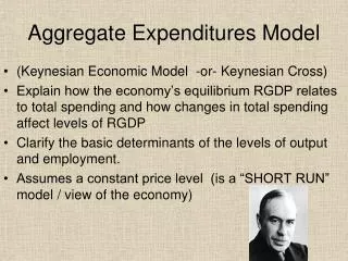
The Goods Market and the Aggregate Expenditures Model. Chapter 8. The Historical Development of Modern Macroeconomics. The Great Depression of the 1930s led to the development of macroeconomics and aggregate demand tools to deal with recessions.

E N D
The Goods Market and the Aggregate Expenditures Model Chapter 8
The Historical Development of Modern Macroeconomics • The Great Depression of the 1930s led to the development of macroeconomics and aggregate demand tools to deal with recessions. • During the Depression, output fell by 30 percent and unemployment rose to 25 percent.
Equilibrium Income Fluctuates • Equilibrium income – the level toward which the economy gravitates in the short run because of the cumulative cycles of declining or increasing production.
Equilibrium Income Fluctuates • Potential income – the level of income that the economy technically is capable of producing without generating accelerating inflation.
The Paradox of Thrift • Paradox of thrift – an increase in savings can lead to a decrease in expenditures, decreasing output and causing a recession.
Aggregate Production • Aggregate production –the total amount of goods and services produced in every industry in an economy. • Production creates an equal amount of income. • Thus, actual production and actual income are always equal.
Aggregate production (production = income) Real production C A $4,000 Potential income 45º 0 $4,000 Real income The Aggregate Production Curve
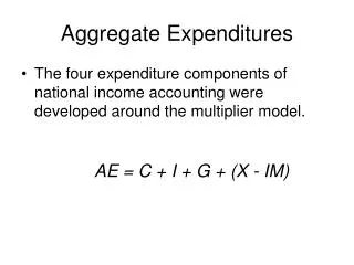
Aggregate Expenditures • Aggregateexpenditures – the total amount of spending on final goods and services in the economy: • Consumption – spending by households. • Investment – spending by business. • Spending by government. • Net foreign spending on Canadian goods – the difference between Canadian exports and imports.
Autonomous and Induced Expenditures • Autonomous expenditures are expenditures that are independent of income. • Autonomous expenditures change because something other than income changes. • Induced expenditures – expenditures that change as income changes.
The Expenditures Function • The relationship between aggregate expenditures and income can be expressed mathematically: AE = AEo + mpcY AE = aggregate expenditures AEo = autonomous expenditures mpc = marginal propensity to consume Y = income
The Marginal Propensity to Consume • Marginal propensity to consume (mpc) – the change in consumption that occurs with a change in income. • The mpc is between 0 and 1 because individuals tend to save a portion of an increase in income.
The Marginal Propensity to Consume • The mpc is the fraction spent from an additional dollar of income.
Aggregate production AE = 1,000 + 0.8Y AE = 2,000 Y = 2,500 45º $8,750 $11,250 $14,000 Graphing the Expenditures Function $12,200 10,000 8,000 Real expenditures (AE) 6,000 5,000 4,000 2,000 1,000 0 $5,000 Real income
Shifts in the Expenditures Function • The aggregate expenditure curve shifts when autonomous C, I, G, or (X – IM) change. • Autonomous Consumption expenditures respond to changes in: • interest rates • household wealth • expectations of future conditions
Shifts in the Expenditures Function • Autonomous Investment is the most volatile component of GDP. • It responds to changes in: • interest rates • capital goods prices • consumer demand conditions • expectations regarding future economic conditions
Shifts in the Expenditures Function • Autonomous exports and imports depend on foreign and domestic incomes and relative prices. • Autonomous Government expenditures may also change as policies change.
Determining the Equilibrium Level of Aggregate Income • At equilibrium, planned expenditures must equal production. • Graphically, it is the income level at which AE equals AP.
Aggregate production $14,000 Aggregate expenditures 12,200 10,000 Real expenditures (AE) 8,000 5,000 2,600 AE0 = $1,000 1,000 45° 0 $2,000 $5,000 $10,000 $14,000 Real income Solving for Equilibrium Graphically AE = 1,000 + 0.8Y E
Aggregate production A1 Aggregate expenditures A2 C B1 B2 45° The Multiplier Process C, I, G, (X – IM) $14,000 $13,200 AE = 1,000 + 0.8Y 10,000 Real expenditures (AE) 6,000 2,000 0 $2,000 $5,000 $10,000 $14,000 Real income
The Circular Flow Model and the Multiplier Process • Expenditures are injections into the circular flow. • The mpc measures the percentage of expenditures that get injected back into the economy each round of the circular flow. • But there are withdrawals.
The Circular Flow Model and the Multiplier Process • Economists use the term the marginal propensity of save (mps) to represent the percentage of income flow that is withdrawn from the economy for each round of the circular flow.
The Circular Flow Model and the Multiplier Process • By definition: mpc + mps = 1 • Alternatively expressed: mps = 1 - mpc multiplier = 1/mps
Aggregate income Households Firms Aggregate expenditures The Circular Flow Model and the Multiplier Process
Examples of the Effect of Shifts in Aggregate Expenditures • There are many reasons for shifts in autonomous expenditures: • Natural disasters. • Changes in investment caused by technological developments. • Shifts in government expenditures. • Large changes in the exchange rate.
Real expenditures Aggregate production AE1 $4,210 30 AE0 4,090 1,052.5 30 1,022.5 $120 0 $4,090 $4,210 Real income Upward Shift of AE
Aggregate production AE0 $4,152 AE1 30 4,062 30 1,412 1,382 $90 $4,062 $4,152 Downward Shift of AE Real expenditures 0 Real income
Model of Aggregate Demand • Shifts may be simultaneous shifts in supply and demand that do not necessarily reflect suppliers' responding to changes in demand. • Expansion of this line of thought has led to the real business cycle theory of the economy.
Model of Aggregate Demand • Real business cycle theory of the economy – changes in aggregate supply are the principle way for real income to change.
Prices are Fixed • The multiplier model assumes that the price level is fixed. • The price level can change in response to changes in aggregate demand.
Forward-Looking Expectations Complicate the Adjustment Process • Rational expectations model – captures the effect expectations have on individuals’ behaviour. • Expectations can be self-fulfilling.
Consumption Behaviour • People may base their spending on lifetime income, not yearly income. • Permanent income hypothesis -- the hypothesis that expenditures are determined by permanent or lifetime income.
Expanded AE Model • We can increase the power of our AE model by adding more detail. • For example, adding taxes to the model • Changes consumption expenditures. • Introduces government budget deficits and surpluses. • Changes the multiplier.
Budget Surplus Function Budget Surplus T - G 0 Income
Expanded AE Model • Adding income-induced imports • Changes import spending. • Changes net exports, • and introduces trade surpluses and deficits. • Changes the multiplier.
Expanded AE Model • The marginal propensity to import (mpi) gives the increase in import spending from an additional $1 of disposable income. • Disposable = after-tax • Mpi lies between 0 and 1
The Goods Market and the Aggregate Expenditures Model End of Chapter 8