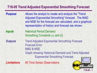
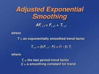
Adjusted Exponential Smoothing
Adjusted Exponential Smoothing. AF t +1 = F t +1 + T t +1 where T = an exponentially smoothed trend factor T t +1 = ( F t +1 - F t ) + (1 - ) T t where T t = the last period trend factor = a smoothing constant for trend. Adjusted Exponential Smoothing Example.

Adjusted Exponential Smoothing
E N D
Presentation Transcript
Adjusted Exponential Smoothing AFt +1 = Ft +1 + Tt +1 where T = an exponentially smoothed trend factor Tt +1 = (Ft +1 - Ft) + (1 - ) Tt where Tt= the last period trend factor = a smoothing constant for trend
PERIOD MONTH DEMAND 1 Jan 37 2 Feb 40 3 Mar 41 4 Apr 37 5 May 45 6 Jun 50 7 Jul 43 8 Aug 47 9 Sep 56 10 Oct 52 11 Nov 55 12 Dec 54 Adjusted Exponential Smoothing Example
PERIOD MONTH DEMAND 1 Jan 37 2 Feb 40 3 Mar 41 4 Apr 37 5 May 45 6 Jun 50 7 Jul 43 8 Aug 47 9 Sep 56 10 Oct 52 11 Nov 55 12 Dec 54 T3 = (F3 - F2) + (1 - ) T2 = (0.30)(38.5 - 37.0) + (0.70)(0) = 0.45 AF3 = F3 + T3 = 38.5 + 0.45 = 38.95 T13 = (F13 - F12) + (1 - ) T12 = (0.30)(53.61 - 53.21) + (0.70)(1.77) = 1.36 AF13 = F13 + T13 = 53.61 + 1.36 = 54.96 Adjusted Exponential Smoothing Example
Adjusted Exponential Smoothing Example FORECAST TREND ADJUSTED PERIOD MONTH DEMAND Ft +1 Tt +1 FORECAST AFt +1 1 Jan 37 37.00 – – 2 Feb 40 37.00 0.00 37.00 3 Mar 41 38.50 0.45 38.95 4 Apr 37 39.75 0.69 40.44 5 May 45 38.37 0.07 38.44 6 Jun 50 38.37 0.07 38.44 7 Jul 43 45.84 1.97 47.82 8 Aug 47 44.42 0.95 45.37 9 Sep 56 45.71 1.05 46.76 10 Oct 52 50.85 2.28 58.13 11 Nov 55 51.42 1.76 53.19 12 Dec 54 53.21 1.77 54.98 13 Jan – 53.61 1.36 54.96
70 – 60 – 50 – 40 – 30 – 20 – 10 – 0 – Demand | | | | | | | | | | | | | 1 2 3 4 5 6 7 8 9 10 11 12 13 Period Adjusted Exponential Smoothing Forecasts
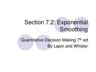
70 – 60 – 50 – 40 – 30 – 20 – 10 – 0 – Actual Demand Forecast ( = 0.50) | | | | | | | | | | | | | 1 2 3 4 5 6 7 8 9 10 11 12 13 Period Adjusted Exponential Smoothing Forecasts
70 – 60 – 50 – 40 – 30 – 20 – 10 – 0 – Adjusted forecast ( = 0.30) Actual Demand Forecast ( = 0.50) | | | | | | | | | | | | | 1 2 3 4 5 6 7 8 9 10 11 12 13 Period Adjusted Exponential Smoothing Forecasts
Linear Trend Line y = a + bx where a = intercept (at period 0) b = slope of the line x = the time period y = forecast for demand for period x
xy - nxy x2- nx2 b = a = y - b x where n = number of periods x = = mean of the x values y = = mean of the y values x n y n Linear Trend Line y = a + bx where a = intercept (at period 0) b = slope of the line x = the time period y = forecast for demand for period x
x(PERIOD) y(DEMAND) 1 73 2 40 3 41 4 37 5 45 6 50 7 43 8 47 9 56 10 52 11 55 12 54 78 557 Least Squares Example
x(PERIOD) y(DEMAND) xy x2 1 73 37 1 2 40 80 4 3 41 123 9 4 37 148 16 5 45 225 25 6 50 300 36 7 43 301 49 8 47 376 64 9 56 504 81 10 52 520 100 11 55 605 121 12 54 648 144 78 557 3867 650 Least Squares Example
x(PERIOD) y(DEMAND) xy x2 557 12 78 12 1 73 37 1 2 40 80 4 3 41 123 9 4 37 148 16 5 45 225 25 6 50 300 36 7 43 301 49 8 47 376 64 9 56 504 81 10 52 520 100 11 55 605 121 12 54 648 144 78 557 3867 650 x = = 6.5 y = = 46.42 b = = = 1.72 a = y - bx = 46.42 - (1.72)(6.5) = 35.2 xy - nxy x2 - nx2 3867 - (12)(6.5)(46.42) 650 - 12(6.5)2 Least Squares Example
Linear trend line x(PERIOD) y(DEMAND) xy x2 y = 35.2 + 1.72x 557 12 78 12 1 73 37 1 2 40 80 4 3 41 123 9 4 37 148 16 5 45 225 25 6 50 300 36 7 43 301 49 8 47 376 64 9 56 504 81 10 52 520 100 11 55 605 121 12 54 648 144 78 557 3867 650 x = = 6.5 y = = 46.42 b = = = 1.72 a = y - bx = 46.42 - (1.72)(6.5) = 35.2 xy - nxy x2 - nx2 3867 - (12)(6.5)(46.42) 650 - 12(6.5)2 Least Squares Example
x(PERIOD) y(DEMAND) xy x2 Linear trend line 557 12 78 12 1 73 37 1 2 40 80 4 3 41 123 9 4 37 148 16 5 45 225 25 6 50 300 36 7 43 301 49 8 47 376 64 9 56 504 81 10 52 520 100 11 55 605 121 12 54 648 144 78 557 3867 650 x = = 6.5 y = = 46.42 b = = = 1.72 a = y - bx = 46.42 - (1.72)(6.5) = 35.2 y = 35.2 + 1.72x Forecast for period 13 y = 35.2 + 1.72(13) xy - nxy x2 - nx2 3867 - (12)(6.5)(46.42) 650 - 12(6.5)2 y = 57.56 units Least Squares Example
70 – 60 – 50 – 40 – 30 – 20 – 10 – 0 – Demand | | | | | | | | | | | | | 1 2 3 4 5 6 7 8 9 10 11 12 13 Period Linear Trend Line
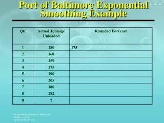
70 – 60 – 50 – 40 – 30 – 20 – 10 – 0 – Actual Demand | | | | | | | | | | | | | 1 2 3 4 5 6 7 8 9 10 11 12 13 Period Linear Trend Line
70 – 60 – 50 – 40 – 30 – 20 – 10 – 0 – Actual Demand Linear trend line | | | | | | | | | | | | | 1 2 3 4 5 6 7 8 9 10 11 12 13 Period Linear Trend Line
Seasonal Adjustments • Repetitive increase/ decrease in demand • Use seasonal factor to adjust forecast
Di D Seasonal factor = Si = Seasonal Adjustments • Repetitive increase/ decrease in demand • Use seasonal factor to adjust forecast
DEMAND (1000’S PER QUARTER) YEAR 1 2 3 4 Total 1999 12.6 8.6 6.3 17.5 45.0 2000 14.1 10.3 7.5 18.2 50.1 2001 15.3 10.6 8.1 19.6 53.6 Total 42.0 29.5 21.9 55.3 148.7 Seasonal Adjustment
DEMAND (1000’S PER QUARTER) YEAR 1 2 3 4 Total 1999 12.6 8.6 6.3 17.5 45.0 2000 14.1 10.3 7.5 18.2 50.1 2001 15.3 10.6 8.1 19.6 53.6 Total 42.0 29.5 21.9 55.3 148.7 42.0 148.7 29.5 148.7 55.3 148.7 21.9 148.7 D1 D D2 D D4 D D3 D S1 = = = 0.28 S2 = = = 0.20 S4 = = = 0.37 S3 = = = 0.15 Seasonal Adjustment
DEMAND (1000’S PER QUARTER) YEAR 1 2 3 4 Total 1999 12.6 8.6 6.3 17.5 45.0 2000 14.1 10.3 7.5 18.2 50.1 2001 15.3 10.6 8.1 19.6 53.6 Total 42.0 29.5 21.9 55.3 148.7 Si 0.28 0.20 0.15 0.37 Seasonal Adjustment
DEMAND (1000’S PER QUARTER) YEAR 1 2 3 4 Total 1999 12.6 8.6 6.3 17.5 45.0 2000 14.1 10.3 7.5 18.2 50.1 2001 15.3 10.6 8.1 19.6 53.6 Total 42.0 29.5 21.9 55.3 148.7 Si 0.28 0.20 0.15 0.37 Seasonal Adjustment For 2002 y = 40.97 + 4.30x = 40.97 + 4.30(4) = 58.17
DEMAND (1000’S PER QUARTER) YEAR 1 2 3 4 Total 1999 12.6 8.6 6.3 17.5 45.0 2000 14.1 10.3 7.5 18.2 50.1 2001 15.3 10.6 8.1 19.6 53.6 Total 42.0 29.5 21.9 55.3 148.7 Si 0.28 0.20 0.15 0.37 Seasonal Adjustment For 2002 y = 40.97 + 4.30x = 40.97 + 4.30(4) = 58.17 SF1 = (S1) (F5) SF3 = (S3) (F5) = (0.28)(58.17) = 16.28 = (0.15)(58.17) = 8.73 SF2 = (S2) (F5) SF4 = (S4) (F5) = (0.20)(58.17) = 11.63 = (0.37)(58.17) = 21.53
Forecast Accuracy • Error = Actual - Forecast • Find a method which minimizes error • Mean Absolute Deviation (MAD) • Mean Absolute Percent Deviation (MAPD) • Cumulative Error (E)
Dt - Ft n MAD = Mean Absolute Deviation (MAD) where t = the period number Dt = demand in period t Ft = the forecast for period t n = the total number of periods = the absolute value
PERIOD DEMAND, DtFt ( =0.3) 1 37 37.00 2 40 37.00 3 41 37.90 4 37 38.83 5 45 38.28 6 50 40.29 7 43 43.20 8 47 43.14 9 56 44.30 10 52 47.81 11 55 49.06 12 54 50.84 557 MAD Example
PERIOD DEMAND, DtFt ( =0.3) (Dt - Ft) |Dt - Ft| 1 37 37.00 – – 2 40 37.00 3.00 3.00 3 41 37.90 3.10 3.10 4 37 38.83 -1.83 1.83 5 45 38.28 6.72 6.72 6 50 40.29 9.69 9.69 7 43 43.20 -0.20 0.20 8 47 43.14 3.86 3.86 9 56 44.30 11.70 11.70 10 52 47.81 4.19 4.19 11 55 49.06 5.94 5.94 12 54 50.84 3.15 3.15 557 49.31 53.39 MAD Example
PERIOD DEMAND, DtFt ( =0.3) (Dt - Ft) |Dt - Ft| 1 37 37.00 – – 2 40 37.00 3.00 3.00 3 41 37.90 3.10 3.10 4 37 38.83 -1.83 1.83 5 45 38.28 6.72 6.72 6 50 40.29 9.69 9.69 7 43 43.20 -0.20 0.20 8 47 43.14 3.86 3.86 9 56 44.30 11.70 11.70 10 52 47.81 4.19 4.19 11 55 49.06 5.94 5.94 12 54 50.84 3.15 3.15 557 49.31 53.39 • Dt - Ft n MAD = = = 4.85 53.39 11 MAD Example
Mean absolute percent deviation (MAPD) MAPD = |Dt - Ft| Dt • Cumulative error E = et et n • Average error E = Other Accuracy Measures
FORECAST MAD MAPD E (E) Exponential smoothing (= 0.30) 4.85 9.6% 49.31 4.48 Exponential smoothing (= 0.50) 4.04 8.5% 33.21 3.02 Adjusted exponential smoothing 3.81 8.1% 21.14 1.92 (= 0.50, = 0.30) Linear trend line 2.29 4.9% – – Comparison of Forecasts
Forecast Control • Reasons for out-of-control forecasts • Change in trend • Appearance of cycle • Weather changes • Promotions • Competition • Politics
(Dt - Ft) MAD E MAD Tracking signal = = Tracking Signal • Compute each period • Compare to control limits • Forecast is in control if within limits Use control limits of +/- 2 to +/- 5 MAD
DEMAND FORECAST, ERROR E = PERIOD DtFtDt - Ft(Dt - Ft) MAD 1 37 37.00 – – – 2 40 37.00 3.00 3.00 3.00 3 41 37.90 3.10 6.10 3.05 4 37 38.83 -1.83 4.27 2.64 5 45 38.28 6.72 10.99 3.66 6 50 40.29 9.69 20.68 4.87 7 43 43.20 -0.20 20.48 4.09 8 47 43.14 3.86 24.34 4.06 9 56 44.30 11.70 36.04 5.01 10 52 47.81 4.19 40.23 4.92 11 55 49.06 5.94 46.17 5.02 12 54 50.84 3.15 49.32 4.85 Tracking Signal Values
DEMAND FORECAST, ERROR E = PERIOD DtFtDt - Ft(Dt - Ft) MAD 1 37 37.00 – – – 2 40 37.00 3.00 3.00 3.00 3 41 37.90 3.10 6.10 3.05 4 37 38.83 -1.83 4.27 2.64 5 45 38.28 6.72 10.99 3.66 6 50 40.29 9.69 20.68 4.87 7 43 43.20 -0.20 20.48 4.09 8 47 43.14 3.86 24.34 4.06 9 56 44.30 11.70 36.04 5.01 10 52 47.81 4.19 40.23 4.92 11 55 49.06 5.94 46.17 5.02 12 54 50.84 3.15 49.32 4.85 6.10 3.05 Tracking signal for period 3 TS3 = = 2.00 Tracking Signal Values
DEMAND FORECAST, ERROR E = TRACKING PERIOD DtFtDt - Ft(Dt - Ft) MAD SIGNAL 1 37 37.00 – – – – 2 40 37.00 3.00 3.00 3.00 1.00 3 41 37.90 3.10 6.10 3.05 2.00 4 37 38.83 -1.83 4.27 2.64 1.62 5 45 38.28 6.72 10.99 3.66 3.00 6 50 40.29 9.69 20.68 4.87 4.25 7 43 43.20 -0.20 20.48 4.09 5.01 8 47 43.14 3.86 24.34 4.06 6.00 9 56 44.30 11.70 36.04 5.01 7.19 10 52 47.81 4.19 40.23 4.92 8.18 11 55 49.06 5.94 46.17 5.02 9.20 12 54 50.84 3.15 49.32 4.85 10.17 Tracking Signal Values
3 – 2 – 1 – 0 – -1 – -2 – -3 – Tracking signal (MAD) | | | | | | | | | | | | | 0 1 2 3 4 5 6 7 8 9 10 11 12 Period Tracking Signal Plot
3 – 2 – 1 – 0 – -1 – -2 – -3 – Exponential smoothing ( = 0.30) Tracking signal (MAD) | | | | | | | | | | | | | 0 1 2 3 4 5 6 7 8 9 10 11 12 Period Tracking Signal Plot
3 – 2 – 1 – 0 – -1 – -2 – -3 – Exponential smoothing ( = 0.30) Tracking signal (MAD) Linear trend line | | | | | | | | | | | | | 0 1 2 3 4 5 6 7 8 9 10 11 12 Period Tracking Signal Plot
= (Dt - Ft)2 n - 1 Statistical Control Charts • Using we can calculate statistical control limits for the forecast error • Control limits are typically set at 3
18.39– 12.24– 6.12– 0– -6.12– -12.24– -18.39– | | | | | | | | | | | | | 0 1 2 3 4 5 6 7 8 9 10 11 12 Period Statistical Control Charts Errors
18.39– 12.24– 6.12– 0– -6.12– -12.24– -18.39– UCL = +3 LCL = -3 | | | | | | | | | | | | | 0 1 2 3 4 5 6 7 8 9 10 11 12 Period Statistical Control Charts Errors
Causal Modeling with Linear Regression • Study relationship between two or more variables • Dependent variable y depends on independent variable xy = a + bx
a = y - b x b = where a = intercept (at period 0) b = slope of the line x = = mean of the x data y = = mean of the y data xy - nxy x2- nx2 x n y n Linear Regression Formulas
x y (WINS) (ATTENDANCE) xyx2 4 36.3 145.2 16 6 40.1 240.6 36 6 41.2 247.2 36 8 53.0 424.0 64 6 44.0 264.0 36 7 45.6 319.2 49 5 39.0 195.0 25 7 47.5 332.5 49 49 346.7 2167.7 311 Linear Regression Example
x y (WINS) (ATTENDANCE) xyx2 4 36.3 145.2 16 6 40.1 240.6 36 6 41.2 247.2 36 8 53.0 424.0 64 6 44.0 264.0 36 7 45.6 319.2 49 5 39.0 195.0 25 7 47.5 332.5 49 49 346.7 2167.7 311 x = = 6.125 y = = 43.36 b= = = 4.06 a= y - bx = 43.36 - (4.06)(6.125) = 18.46 49 8 xy - nxy2 x2 - nx2 346.9 8 (2,167.7) - (8)(6.125)(43.36) (311) - (8)(6.125)2 Linear Regression Example
x y (WINS) (ATTENDANCE) xyx2 4 36.3 145.2 16 6 40.1 240.6 36 6 41.2 247.2 36 8 53.0 424.0 64 6 44.0 264.0 36 7 45.6 319.2 49 5 39.0 195.0 25 7 47.5 332.5 49 49 346.7 2167.7 311 x = = 6.125 y = = 43.36 b= = = 4.06 a= y - bx = 43.36 - (4.06)(6.125) = 18.46 49 8 Regression equation xy - nxy2 x2 - nx2 346.9 8 y = 18.46 + 4.06x Attendance forecast for 7 wins (2,167.7) - (8)(6.125)(43.36) (311) - (8)(6.125)2 y = 18.46 + 4.06(7) = 46.88, or 46,880 Linear Regression Example
Attendance, y | | | | | | | | | | | 0 1 2 3 4 5 6 7 8 9 10 Wins, x Linear Regression Line 60,000 – 50,000 – 40,000 – 30,000 – 20,000 – 10,000 –