Cycles and Exponential Smoothing Models

1. Cycles and Exponential Smoothing Models • Materials for this lecture • Lecture 4 Cycles.XLS • Lecture 4 Exponential Smoothing.XLS • Read Chapter 15 pages 18-30 • Read Chapter 16 Section 14

2. How Good is Your Forecast? • Can your forecast beat a Moving Average? • Business forecasters use Moving Average as a point of comparison • MAPE for MA model • MAPE for your model • Example of two Data Series • X with a Moving Average MAPE of 23% • Your model’s MAPE of 15% • Y with a Moving Average MAPE of 12% • Your model’s MAPE of 10%

3. Cycles, Seasonal Decomposition and Exponential Smoothing Models • Business cycle • Beef cycle • Hog cycle • Weather cycle? • Cycles caused by over correction of an economic system • The Cob Web Theorem in action

4. Cycles and Exponential Smoothing Models • Cyclical analysis involves analyzing data for underlying cycles • Estimate length of cycle • Forecast variable based on cycle length • Exponential Smoothing most often used forecasting method in industry • Easy to use and update, very flexible • Only forecasts a few periods ahead is major disadvantage

5. Cyclical Analysis Models • Harmonic regression model estimated with OLS regression estimates cycle length • Sin and Cos using CL variable • Need enough observations to see several cycles in the data series • Two considerations in estimating cycle length and specifying the OLS model • Annual data can easily exhibit a cycle • Monthly data can show a seasonal pattern about a multiple year cycle

6. Cyclical Analysis Models • If you are using Annual data • Define CL = Number of years for a possible cycle length, as CL = 5 to test for a 5 year cycle • If you are using Monthly data • Define CL = SL * No. Years for cycle length where SL = 12 number of months in a year • If you are using Quarterly data • Define SL = 4 number of quarters in a year

7. Cyclical Analysis Models • OLS regression model for annual data Ŷ = a + b1T + b2 Sin(2*ρi*T/CL) + b3 Cos(2*ρi*T/CL) where: CL is the number of years for a cycle • Estimate the best cycle length • Enter CL in a cell • Refer to the cell with CL to calculate the Sin() and Cos() values in the X matrix • Estimate regression model in Simetar for a CL • Change the value for CL, observe the MAPE • Change the value for CL, observe the MAPE • Repeat process for numerous CL values and find the CL with the lowest MAPE

8. Cyclical Analysis Models • OLS regression model for monthly data Ŷ = a +b1T+ b2Sin(2*ρi*T/SL) + b3Cos(2*ρi*T/SL) + b4Sin(2*ρi*T/CL) + b5Cos(2*ρi*T/CL) where SL = No. months (quarters, or weeks) in a year and CL = SL * No. years for a cycle • Estimate the best cycle length • Enter the No. Years in a cell • Calculate CL in a cell with CL = SL * Years • Refer to the cell with CL to calculate the second Sin() and Cos() values in X matrix • Estimate regression model in Simetar for No. of Years • Change the CL value for no. of years in cycle, observe the MAPE • Repeat process for different CL values for No. of years and pick the CL for the lowest MAPE

9. Cyclical Analysis Models • Part of the Y and X matrix for annual data • Sin and Cos functions refer to CL in C49

10. Cyclical Analysis Models • Y and X matrix for a monthly data series • Sin and Cos functions refer to CL and SL in C11 and F11 Lecture 4

11. Cyclical Analysis Models • Sample table of R2 and MAPE for CL’s • CL = 9 for the chart and regression shown here, based on maximum MAPE

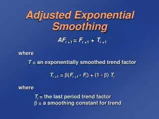
12. Exponential Smoothing Models • ES is the most popular forecasting method • Very good for forecasting a few periods • Like moving average, but greater weights placed on more recent observations • Level for period T LT = a YT + (1-a) LT-1 where a is the smoothing constant ŶT+1 = LT = a YT + (1-a) LT-1

13. Exponential Smoothing Models • Different forms of ES models 1. Simple exponential smoothing, additive seasonal and no trend (1 seasonal ,0 trend) 2. Additive seasonal and additive trend (1,1) 3. Additive trend and multiplicative seasonal variability (2,1) 4. Multiplicative trend and multiplicative seasonal variability (2,2) 5. Dampened trend ES with additive seasonal variability (1,1) 6. Dampened trend ES with multiplicative seasonal variability (2,2) • Numbers match chart numbers in next two slides • Numbers in ()’s match Simetar ES option settings

14. Exponential Smoothing Models 2. Additive seasonal variability with an additive trend (1,1) 1. No trend and additive seasonal variability (1,0) 3. Multiplicative seasonal variability with an additive trend (2,1) 4. Multiplicative seasonal variability with a multiplicative trend (2,2)

15. Exponential Smoothing Models • Select the type of model to fit based on the presence of • Trend – additive or multiplicative, dampened or not • Seasonal variability – additive or multiplicative • Do this prior to the estimation. With Simetar you can experiment with different specifications after model is estimated • Can select 3 seasonal effects: none, additive, multiplicative • Can select 3 trend effects: none, additive, multiplicative 5. Dampened trend with additive seasonal variability (1,1) 6. Multiplicative seasonal variability and dampened trend (2,2)

16. Exponential Smoothing Forecasts • Using the Forecasting Icon for ES • Data on the Excel toolbar to get Data Ribbon • Select Solver • Close Solver • Select the “Exponential Smoothing” tab in Simetar • Specify the data series to forecast • Provide initial guesses for • Dampening Factor (0.5), • Trend Factor (0.5), and • Season Factor (0.5) • Indicate the Optional Seasons per Period as 12 • Forecast Periods of 1 or 6

17. Exponential Smoothing Models • Simetar estimates all forms of ES models • Provides deterministic forecasts • Provides probabilistic forecasts • Parameters for ES model estimated by Solver to minimize MAPE for residuals • PRIOR to running ES MUST open Solver and close it • Provide starting guesses for parameters 0.25 to 0.50 • Enter no. of periods/year

18. Exponential Smoothing Models • Initial Parameters for ES • Dampening Factor is required for all models – good guess is 0.25 • Optional Trend factor entered as 0.5 if the data have any trend • Optional Seasonal factor, 0.5, if the data are monthly or you have >30 years annual data (with annual data you have a cycle) • Optional Seasons per Period • Indicate the number of months for seasonal effect as 12 • Indicate cycle length if using annual data, say 9 years

19. Exponential Smoothing Models • ES Options • Season Method • 0 No seasonal effects • 1 Additive seasonal effect • 2 Multiplicative seasonal effect • Trend Method • 0 No trend dampening • 1 Dampened Additive • 2 Dampened Multiplicative • Stochastic Forecast • TRUE • FALSE

20. Exponential Smoothing Models • Experiment with alternative settings for the Trend and Seasonal Smoothing variables to see which combination is best • Look for the lowest MAPE

21. Exponential Smoothing Models 2. Additive seasonal variability with an additive trend (1,1) 1. No trend and additive seasonal variability (1,0) 3. Multiplicative seasonal variability with an additive trend (2,1) 4. Multiplicative seasonal variability with a multiplicative trend (2,2)

22. Exponential Smoothing Models • Select the type of model to fit based on the presence of • Trend – additive or multiplicative, dampened or not • Seasonal variability – additive or multiplicative • Do this prior to the estimation. With Simetar you can experiment with different specifications after model is estimated • Can select 3 seasonal effects: none, additive, multiplicative • Can select 3 trend effects: none, additive, multiplicative 5. Dampened trend with additive seasonal variability (1,1) 6. Multiplicative seasonal variability and dampened trend (2,2)