Download
1 / 25
250 likes | 267 Vues
This text outlines the search for volatiles on Saturn's icy moons, detailing observations, methodology, and results for Tethys, Dione, Iapetus, Rhea, and Enceladus. The goals, observations, and findings for each moon are discussed, highlighting the search for potential gas absorption and atmospheric features. The upper limits and lack of evidence for volatiles detected through occultations are summarized.

E N D
Icy Moon Occultations: the Search for Volatiles C. J. Hansen, A. Hendrix, B. Meinke 6 January 2010
Outline • Overview • Tethys • Dione • Iapetus • Rhea • Upper limits • Enceladus Enceladus’ Plume
UVIS Observations of Stellar Occultations Why do we observe occultations of bright stars by Saturn’s icy moons with UVIS? • Typically to look for volatiles • Dione, Rhea, Iapetus • Enceladus’ plume • Sometimes for rings • Rhea • UVIS Configuration: • FUV • 5 sec integration • 512 spectral channels • HSP • 2 msec integration Sigma SGR over Iapetus
Methodology Step 1: Plot HSP data. The ingress is clean - this is the first place to look for any attenuation. The egress is plagued by the instrument signal coming up again, so apparent dips on egress are artifacts. To look for attenuation on egress must sum FUV over wavelength, but this means temporal resolution is 5 sec, not 2 msec. Step 2: Determine which spatial rows of the FUV the star is in and sum over those rows. Generate I0 spectrum, the unocculted signal, pre-ingress and post-egress. Plot potentially occulted signal I, with I0, to compare. Step 3: Plot I / I0 to see absorption features. In the case of Tethys, Rhea, Iapetus, and Dione we have found none. In the case of Enceladus we clearly see absorption by water vapor by the plume. Step 4: If absorption features are detected model gas column density and compare gas absorption features to I / I0 Step 5: If no absorption features, calculate upper limits
Tethys Goal: Search for volatiles in Tethys’ vicinity. Use this airless body to compare others with more potential for gases. Result: No evidence for gas absorption (as expected) Occultations Observed Orbit 15 2005-267T02:36 beta Tau Orbit 24 2006-143T04:32 66 Oph Orbit 27 2006-235T23:21 8 nu Cap Orbit 15
Dione Goal: Search for volatiles - MAPS instruments detect mass-loading of magnetosphere near Dione, similar to Enceladus but down more than an order of magnitude? Look for small plumes. May be very localized. Result: No evidence for gas absorption (yet) Occultations Observed Observation start Star Ingress lat/long Egress lat/long Orbit 19 2005-358T16:40 66 Oph -53.8 / 148.1 -52.4 / 327.9 Orbit 45 2007-147T12:12 alpha Leo 48.5 / 94.9 61.9 / 304.3 Orbit 118 2009-263T17:00 epsilon Cma 11.5 / 2.5 26.3 / 163.1 Orbit 19
Dione Orbit 45 Counts / 100 msec Orbit 118
Iapetus Goal: Search for volatiles possibly being transported from the dark side to the bright side of Iapetus - MAPS instruments report that Iapetus has interesting / unusual interaction with solar wind. Result: No evidence for gas absorption Occultation Observed Orbit 49 2007-253T12:55 sigma SGR
Rhea Goal: Search for oxygen atmosphere that could cause plasma absorption detected by MIMI. Search for ring material that could cause plasma absorption detected by MIMI. Only moon massive enough to retain a sputtered atmosphere • Recall: • Cassini’s flyby of Rhea in November 2005 was through the wake - a region in which a depletion in charged particles is expected • The expected depletion was detected, but over a larger expanse than predicted • MIMI observed a depletion of energetic electrons - their interpretation is that it is due to a dust cloud, a neutral atmosphere or a combination of both - estimate of required column density is 3 x 1016 cm-2 • MIMI also saw narrow dips in electron flux, attributed possibly to rings Potential ring radii: 1610 km 1800 km 2020 km
Rhea Occultations Observed Orbit 47 2007-179T13:30 eps Ori Orbit 121 2009-325T16:37 beta, kappa Ori Also, non-occultation data was analyzed to look for oxygen emission Orbit 47
Rhea Rev 121 Beta Ori Occultation Rev 121 features a beta Ori occultation ingress and partial egress, and a kappa Ori occultation egress • Ingress was close to equatorial • HSP data doesn’t show any obvious dips
Rhea Rev 121 Beta Ori Egress • Egress was at +80 latitude • Only one of the possible ring locations was crossed by the star
Rhea Kappa Ori Occultation Egress • HSP data, not equatorial • FUV data not analyzed yet Bonnie Meinke ran her software to check for statistically significant dips that could be attributed to rings - none found in this observation -> no confirmation of rings
Rhea Oxygen Emission Results • Rhea does not appear to have a neutral oxygen atmosphere • Although 1304 and 1356 can be well above the background this occurs at geometries where Rhea is viewed close to Enceladus • This allows us to calculate upper limits for O and O2 associated with Rhea, based on not seeing emission features • O: for a 90 min observation, calculated for solar scattering at Saturn, gives an upper limit of 4 x 1013 cm-2 • O2: for a 90 min observation, calculated for electron-impact excitation, gives an upper limit of 1.5 x 1014 cm-2 • The component broadening Rhea’s wake is not a sputtered O or O2 atmosphere
Summary Since no volatiles have been detected in occultations we can calculate upper limits • Calculation of column density upper limits: I0 () exp {-n()}d I/I0 = I0()d • Use I/I0 = 0.95 (reasonable for broad absorptions), plug in absorption crossections as a function of wavelength, solve for n (done numerically, by testing various values of n)
Column Density Upper Limits • All stars we use have a signal high enough to detect a 5% attenuation. This is not adequate for a single absorption feature, however for gases with broad absorptions in the FUV wavelength range it is a realistic threshold. • Gases with absorption features in the FUV: H2O, O2, CO, CO2, NH3, C2H4, methanol • Upper limits • H2O: 2 x 1015 cm-2 • O2: 1.3 x 1015 cm-2 • CO: 3.6 x 1014 cm-2 • CO2: 1.3 x 1017 cm-2 • NH3: 9.2 x 1015 cm-2 • C2H4: 2.8 x 1015 cm-2 • methanol: 4 x 1015 cm-2
Rev 120 Enceladus’ Plume against Saturn
Enceladus Rev 120 • Enceladus flyby on Rev 120 used Saturn as source, looked for Saturn-light absorbed by Enceladus’ plume • Advantage is that plume could potentially be observed more often and over longer time scales than single stellar occultations • “Parked” the slit on Saturn (to minimize changes due to Saturn itself) x 3 • The plume should be resolved horizontally • Reflected uv is not a very strong source however, so it was necessary to sum the data to increase the signal Focus on the data over wavelength range 1646 to 1750 ang, where we have adequate signal from Saturn and a broad absorption feature
Geometer Image: ICYMAP Part 1 • Calibrated data, plot shows 1646 to 1750 ang range • Expect to see plume as darker than Saturn because it is absorbing some of the reflected light
UVIS image of Enceladus’ Plume Range: At start = 18,810 km At end = 32,478 km Resolution: At start = 19 km At end = 32 km ICYMAP Part 1
ICYMAP Part 2 Range: At start = 32,478 km At end = 46,227 km Resolution: At start = 32 km At end = 46 km
ICYMAP Part 3 Range: At start = 46,227 km At end = 57,937 km Resolution: At start = 46 km At end = 57 km
Raw data summed over 1646 to 1750 Range Time • Map shows pixel value divided by column average Orange => pixel 10-20 % lower than average Blue => pixel 20-30% lower than average Lilac => lowest pixel in column Pixels 0 - 61 • Stipples show where plume is • Would like to see correlation of low counts with plume location
Conclusion • This was an experiment worth attempting • But, not clear we can pull out any quantitative results • Standard deviation is ~ equal to the signal we are looking for • Sum more?