Illumination Models

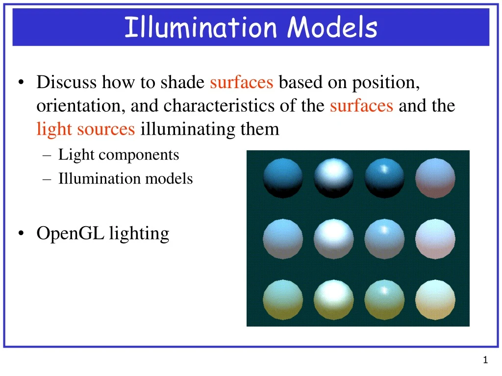
1. Illumination Models • Discuss how to shade surfaces based on position, orientation, and characteristics of the surfaces and the light sources illuminating them • Light components • Illumination models • OpenGL lighting

2. Definitions • Illumination • The transport of energy from a light source to a surface • Lighting • The process of computing the luminous intensity (i.e., outgoing light) at a particular 3D point, usually on a surface • Shading • Assigning colors to pixels

3. Classification of Lights • Lighting is divided into 4 independent components: • Ambient light • Diffuse light • Specular light • Emissive light

4. Ambient Light (1/3) • Ambient illumination is light that’s been scattered so much by the environment that its direction is impossible to determine – it seems to come from all directions • Backlighting in a room has a large ambient component since most of the light reaching your eye has first bounced off many surfaces • A spotlight outdoors has a tiny ambient component since most of the light travels in the same direction

5. Ambient Light (2/3) • Illumination equation: resulting intensity at each point on the object is I = Ia ka • Ia: intensity of the ambient light (light property) • ka: ambient-reflection coefficient, ranging between 0 and 1. (material property)

6. Ambient Light (3/3) • Viewpoint not important • Light position not important • Surface angle not important A sphere lit by a directional light A sphere lit by an ambient light

7. Diffuse Light • The diffuse component is the light that comes from one direction, • so it’s brighter if it comes squarely down on a surface than if it barely glances off the surface • Once it hits the surface, it’s scattered equally in all directions, • so it appears equally bright from all viewing positions

8. Light source Surface normal  Exit surface Lambert’s Law • Brightness depends on the angle  between the light direction and the surface normal • Illumination equation • I = Ip kd cos • Ip: point light intensity • kd: material’s diffuse-reflection coefficient

9. Light-Source Attenuation • Lambertian reflection does not take into account distance between light source and surface points • We introduce a light-source attenuation factor fatt • The energy from a point light source that reaches a given part of a surface falls off as the distance to this part lengthens. • c1, c2, c3 are user-defined constants associated with the light source I = fatt Ip kd cos

10. Specular Light • Specular light comes from a particular direction and tends to bounce the surface in a preferred direction • A well-collimated laser beam bouncing off a mirror produces almost 100% specular reflection • Shiny surface has a high specular component • Chalk and carpet have almost no specular component

11. Surface normal Reflection light Light source View point    Exit surface Phong’s Law I = Is ks cosn • Specular reflection depends on viewpoint: max when  = 0 and falls off as  increases • ks [0, 1]: specular-reflection coefficient, a material property • n  [1, 100’s]: specular-reflection exponent, a material property

12. Putting It All Together #lights Itotal = kaIa +fatt,jIj(kdcosj + kscosnj) j=1 Ambient component Diffuse component Specular component attenuation factor • Usually called Phong Lighting Model • What about colored light???

13. OpenGL Lighting • Define normal vectors for each vertex of every object. These normals determine the orientation of the object relative to the light sources • Create and position light source(s) • Create and select a lighting model: define the level of global ambient light and the effective location of the viewpoint • Define material properties for the objects in the scene

14. Creating a Light Source • void glLight{if}[v](GLenum light, GLenum pname, TYPE param); • light:GL_LIGHT0, GL_LIGHT1, ... , or GL_LIGHT7 • pname: characteristics of the light: GL_AMBIENT, GL_DIFFUSE, GL_SPECULA, GL_POSITION, etc. • param: the value assigned to pname

15. Light Color GLfloat light_ambient[] = { 0.0, 0.0, 0.0, 1.0 }; GLfloat light_diffuse[] = { 1.0, 1.0, 1.0, 1.0 }; GLfloat light_specular[] = { 1.0, 1.0, 1.0, 1.0 }; glLightfv(GL_LIGHT0, GL_AMBIENT, light_ambient); glLightfv(GL_LIGHT0, GL_DIFFUSE, light_diffuse); glLightfv(GL_LIGHT0, GL_SPECULAR, light_specular);

16. Color • Achromatic light • Chromatic color • Color models • Computer color

17. Achromatic Light • What we see on black-and-white monitor or TV • Only 1 attribute: quantity of light. Also called: • intensity, luminance (physics sense of energy) • brightness (psychological sense of perceived intensity) • An achromatic light can be one of different intensity levels between black (0) and white (1) • B/W TV: different intensities at a single pixel • Line printers, pen or electronic plotters: only 2 levels, white (or light gray) and black (or dark gray)

18. Selecting Intensities • Suppose we want n different intensities, how to select them? • I0: lowest attainable intensity • 1: maximum intensity • Therefore, r = (1/I0)1/n • 1/I0 is called dynamic range • Why? • Our eyes are sensitive to ratios of intensity levels rather than to absolute values of intensities • E.g. cycling through a 3-way 50-100-150W bulb, the difference from 50 to 100 seems much greater than that from 100 to 150 CRT monitor: I0 (0.005, 0.025). E.g, if I0 = 0.02, then r = 1.01545.

19. How Many Intensities? • The number of intensities should be chosen so that the reproduction of a continuous-tone B/W image appears continuous • This appearance is achieved when ratio r = (1/I0)1/n is about 1.01. The appropriate value of n therefore is n = log1.01(1/I0)

20. Intensities of Display Media

21. Displaying Intensities • Problem: pixel values are not intensity values. How to display these intensities? • Solution: Gamma Correction • The range of voltages sent to the monitor is between 0 and 1, this means that the intensity value displayed will be less than what you wanted it to be. • To correct this annoying little problem, the input signal to the monitor (the voltage) must be "gamma corrected".

22. Halftone Approximation (1/5) • Problem: • Many displays and hardcopy devices, e.g., in newspaper printing, are bi-level. They produce just two intensity levels. • Even 2- or 3-bit-per-pixel raster displays produce fewer intensity levels than we might desire • Challenge: • How can we expand the range of available intensities to display many intensities? • Solution: • Halftone Approximation

23. Halftone Approximation (2/5) • Each small resolution unit is imprinted with a circle of black ink whose area is proportional to the blackness 1-I of the original area (I = intensity)

24. Halftone Approximation (3/5)

25. Halftone Approximation (4/5) • Graphics output devices can approximate the variable-area circles of halftone reproduction • Use a NxN matrix to produce N2+1 intensity levels

26. Halftone Approximation (5/5) • Dither matrix NxN tells how to display N2+1 intensity level using a NxN group of bilevel pixels 6 8 4 1 0 3 5 2 7 Level 4 Level 5

27. Chromatic Color • Color has 3 quantities: • Hue: distinguishes among colors. E.g., red, green, purple, and yellow • Saturation: how far from a gray of equal intensity. E.g., red is highly saturated, pink is relatively unsaturated • Lightness/Brightness: perceived intensity of a reflecting/self-luminous object

28. Color Perception • Light is composed of photons, each traveling along its own path and vibrating with its own frequencies (or wavelength) • A photon is characterized by position, direction, and frequency/wavelength • Photons with wavelength from 390nm (violet) and 720nm (red) covers the colors of the visible spectrum, forming a rainbow (violet, indigo, blue, green, yellow, orange, red) • Eye perceives a lot more colors. How so? • Mixture of photons.

29. Color Models for Raster Graphics • A color model specifies a color gamut, which is a subset of all visible chromaticities • Hardware-oriented models: not relate to concepts of hue, saturation, and brightness • RGB (red, green, blue): CRT monitors • YMQ: US commercial broadcast TV • CMY (cyan, magenta, yellow): some color-printing devices • User-friendly models: • HSB (hue, saturation, brightness) • HLS (hue, light, saturation) • The Munsell system • CIE lab

30. RGB Models • To display a color, the monitor sends the right proportions of red, green, and blue • Color = a . Red + b . Green + c . Blue • Thus, a color is a point in a color cube

31. Green Yellow (minus blue) (minus red) Cyan Black Red Blue Magenta (minus green) CMY Models • Used in electrostatic and ink-jet plotters that deposit pigment on paper • Cyan, magenta, and yellow are complements of red, green, and blue, respectively • White (0, 0, 0), black (1, 1, 1) • CMYK Model: K (black) is used as a primary color to save ink deposited on paper => dry quicker • popularly used by printing press

32. YIQ Model • Used in US commercial color TV broadcasting • YIQ is a recoding of RGB for transmission efficiency and downward compatibility with B/W TV • Recorded signals are transmitted using the National TV System Committee (NTSV) system • Y: luminance. On B/W TV, only Y is shown • I, Q: chromaticity

33. Computer Color • Computer uses RGB model • Two ways of storing color values for pixels on screen • RGB mode: each pixel associates with one value for R, one for G, and one for B • Color-index mode: each pixel associates with a value, which is an index in the color map <index, RGB values> • Each pixel has the same amount of memory for storing its color; all the memory for all the pixels is called the color buffer • N-bit buffer => N bits of color for each pixel => number of possible colors is 2N • A bitplane contains 1 bit of data for each pixel • Thus, we have N bitplanes

34. RGB Mode vs. Color-Index Mode More colors can be represented by RGB mode If we have a small no. of bitplanes available, RGB may produce noticeably coarse shades of colors while with CIM we can produce only the “good” colors CIM is useful for various tricks, such as color-map animation and drawing in layers

35. Using RGB Color with OpenGL • void glColor3{b s i f d ub us ui} (TYPE r, TYPE g, TYPE b); • Specify a color for drawing the object • void glClearColor(GLclampf red, GLclampf green, GLclampf blue, GLclampf alpha); • Specify a color for clearing the screen • glClearColor(0, 0, 0, 0); // black color • glClear(GL_COLOR_BUFFER_BIT); // clear screen • glColor3f(1.0, 0.0, 0.0); // red color • glBegin(GL_TRIANGLE) // drawing a triangle red color • glVertex2f (5.0, 5.0);         • glVertex2f (25.0, 5.0);         • glVertex2f (5.0, 25.0); • glEnd()

36. Handling Images

37. What is an Image? For our purposes, an image is: • A 2D domain with samples at regular points (usually a rectilinear grid), whose values represent gray levels, colors, or opacities Common image types: • 1 sample per point (B&W or Grayscale) • 3 samples per point (Red, Green, and Blue) • 4 samples per point (Red, Green, Blue, and “Alpha”)

38. Step 1: Image Acquisition • Image synthesis: images are created using a computer. For instance: • images rendered from geometry (e.g., RenderMan, Autodesk 3D Studio) • painted images (e.g., Paint brush, Fractal Design Painter) • Image capture: images that come from the “real world” via scanners, digital cameras, video converter, etc.

39. Step 2: Preprocessing • The source image is adjusted to fit a given tone, size, shape, etc., to match a desired quality or to match some requirements • E.g., make a set of dissimilar images appear similar (if they are to be composited later), or to make similar parts of an image appear dissimilar (such as contrast enhancement) • Preprocessing techniques include: • adjusting color or gray scale curve • cropping • masking (cutting out part of an image to be used in a composition, or to leave a hole in the original image) • scaling up (super sampling)/ down (sub sampling) • blurring and sharpening • edge/enhancement • filtering and antialiasing

40. Step 3: Image Mapping • Several images are combined, or geometric transformations are applied to an image • Transformations include: • rotation • scale • stretch • feature based image warp (a.k.a. morphing) • Compositing: • opaque/transparent paste • alpha-channel composition

41. Step 4: Postprocessing • Used to create global effects across an entire image or selected area(s) • Art effects • Posterizing, faked “aging” of an image, faked “out-of-focus”, “impressionist” pixel remapping, texturizing • Technical effects • color remapping for contrast enhancement, color to B&W conversion, color separation for printing, scan retouching and color/contrast balancing

42. Step 5: Output • How to output the image: to monitor, disks, printer, etc.? • Choice of display/archive method may affect earlier processing stages • color printing accentuates certain colors more than others • colors on the monitor have different gamuts and HSV values than the colors printed out: need a mapping

43. Filtering • After being acquired, the image may have jaggies that make the image not smooth. • Postfiltering: We can replace each pixel value with a weighted sum of itself and its neighbors. E.g., a weighted sum function can be the “average” function. • Rule of thumb (Witted85): • Postfiltering a high-resolution image produces obvious fuzziness but a 2048x2048 image can usually be postfiltered and sampled down to a 512x512 image with good results

44. Scaling an Image • Input: image n x k • Scale factor: p/q (p > q, p and q integers) • Output: image n x (k.p/q) • Problem: if using a scaling function, there will be “black holes” in the target image • Solution: Use Rothstein code

45. Rothstein Code p columns q rows Code = 1 1 0 1 0 Set to 1 because the diagonal line cuts the horizontal segment Belong to column 1

46. Scaling Algorithm char roth[k*p/q]; // repeated rothstein code Loop (p times) { Shift roth 1 bit to right sourceCol = 0; For each column j of output image, if roth[j] = 1 { For each row s: Target[s][j] += source[s][sourceCol] sourceCol ++ } } Divide all the values of target[][] by q End

47. Not yet finished.. • What if p is smaller than q? (scaling to a smaller size) • Only copy from the source image those columns with Rothstein code equal to 1 to the destination image

48. Feibush-Levoy-Cook Algorithm Used for texture mapping on a polygon Source image target These pixels need new values assigned

49. Problem with Feibush-Levoy-Cook • Each target pixel may correspond to a large number of source pixels that need to be transformed and used to compute the filtered value. The computational cost is therefore significant • Other more computationally efficient techniques: • Williams, 1983: MIP map • Crow, 1984: Summed Area Table • Glassner, 1986 • Heckbert 1986

50. MIP MAP (1/2) MIP Map: an image 4/3 bigger in memory than the source image The R, G, B channels of the source contribute 3 quarters of the MIP Map. Each quarter is filtered by a factor of 4 and the three resulting images fill up three quarters of the remaining quarter. The process is continued until the MIP map is filled …