Similarity Flooding
660 likes | 860 Vues
Similarity Flooding. A Versatile Graph Matching Algorithm by Sergey Melnik, Hector Garcia-Molina, Erhard Rahm. Introduction & Motivation. Goal: matching elements of related, complex objects Matching elements of two data schemes Matching elements of two data instances

Similarity Flooding
E N D
Presentation Transcript
Similarity Flooding A Versatile Graph Matching Algorithm by Sergey Melnik, Hector Garcia-Molina, Erhard Rahm Similarity Flooding SDBI – Winter 2001
Introduction & Motivation • Goal: matching elements of related, complex objects • Matching elements of two data schemes • Matching elements of two data instances • Many conceivable uses for object matching • Looking for a generic algorithm with wide applicability Similarity Flooding SDBI – Winter 2001
Applications • Comparing data schemes: • Items from different shopping sites • Merger between two corporations • Preparation of data for data warehousing and analyzing processes • Comparing data instances: • Bio-informatics • Collaboration: allowing multiple users to edit a program / system Similarity Flooding SDBI – Winter 2001
Existing Approaches • Comparing SQL: can use type information • Comparing XML: can use hierarchy Requires domain-specific knowledge and coding Solution: • Generic algorithm that is agnostic to domain • Structural model – relies on structural similarities to find a matching Similarity Flooding SDBI – Winter 2001
Part I: Algorithm Framework General Discussion of Algorithm Input, Output, and Main Components Similarity Flooding SDBI – Winter 2001
Algorithm Framework • Input: two objects to match • Representation of objects as graphs: G1=(V1, E1), G2=(V2, E2) • Matching between graphs gives mapping: V1xV2 • Filtering of mapping to obtain meaningful match • Output: mapping between elements of input objects Human verification sometimes required Similarity Flooding SDBI – Winter 2001
Input Graph Mapping Filtering • Input are two objects to be matched • Match will be between sub-elements of the two objects • Match of sub-elements will be scored. High scores indicate a strong similarity • Assumption: Objects can be represented as graphs Similarity Flooding SDBI – Winter 2001
Input Graph Mapping Filtering • Represent objects as directed, labeled graphs • Choose any sensible graph representation (this is domain-specific) that maintains structural information • Structural information in graphs will be used for mapping. • Intuition: similar elements have similar neighbors G1 = (V1, E1), G2 = (V2, E2) Similarity Flooding SDBI – Winter 2001
Input Graph Mapping Filtering • We want a mapping :V1xV2 • Convenient to normalize such that 0 (v,u) 1 • Begin with initial mapping function: • Null function: (v, u) := 1 for all v in V1, u in V2 • String Matching function • Other domain-specific function • Perform an iterative fixpoint calculation. Each iteration floods the similarity value (v,u) to the neighbors of v and u Similarity Flooding SDBI – Winter 2001
Input Graph Mapping Filtering • We have a mapping :V1xV2 • We are usually not interested in all pairs V1xV2 • Applying filtering functions yields a partial mapping: • Threshold (only when (v,u) > some constant) • Wedding (each v mapped to only one u and vice versa) • Result is a useful mapping that matches elements of V1 with elements of V2 Similarity Flooding SDBI – Winter 2001
Part II: An Example - Relational Schemas An Example Employing the Algorithm to Match Two Simple Relational Schemas Similarity Flooding SDBI – Winter 2001
Example: Relational Schemas • Scenario: two relational schemas that describe similar or same data • Goal: match elements of two given relational schemas • Input: SQL statements for creating each scheme • Desired output: a meaningful mapping between the elements of the two schemas Similarity Flooding SDBI – Winter 2001
CREATE TABLEPersonnel ( Pno int, Pname string, Dept string, Born date, UNIQUEperskey(Pno) ) S1 CREATE TABLEEmployee ( EmpNo int PRIMARY KEY, EmpName varchar(50), DeptNo int REFERENCESDepartment, Salary dec(15,2), Birthdate date ) CREATE TABLE Department ( DeptNo int PRIMARY KEY, DeptName varchar(70) ) S2 Example: Relational SchemasInput Graph Mapping Filtering Similarity Flooding SDBI – Winter 2001
Example: Relational Schemas Algorithm script: G1 = SQLDDL2Graph(S1); G2 = SQLDDL2Graph(S2); initialMap = StringMatch(G1, G2); product = SFJoin(G1, G2, initialMap); result = SelectThreshold(product) Similarity Flooding SDBI – Winter 2001
Example: Relational SchemasInput Graph Mapping Filtering • Any graph representation of schemas can be chosen • Representation should maintain as much information as possible, in particular structural information • Example uses Open Information Model (OIM) – based graph representation Similarity Flooding SDBI – Winter 2001
Example: Relational SchemasInput Graph Mapping Filtering Similarity Flooding SDBI – Winter 2001
Example: Relational SchemasInput Graph Mapping Filtering • Calculate initial mapping to improve performance • Initial mapping can apply domain knowledge • In this example: StringMatch is used: • Compares common prefixes and suffixes of literals • Assumes elements with similar names have similar meaning • Applies on all elements – including elements that are created by the graph representation (e.g. ‘type’) • Initial mapping still far from satisfactory Similarity Flooding SDBI – Winter 2001
Example: Relational SchemasInput Graph Mapping Filtering Similarity Flooding SDBI – Winter 2001
Example: Relational Schemas Input Graph Mapping Filtering • Next step: similarity flooding (SFJoin) • Initial similarity values taken from initial mapping • In each iteration similarity of two elements affects the similarity of their respective neighbors (e.g. similarity of type names such as ‘string’ adds to similarity of columns from the same type) • Iterate until similarity values are stable Similarity Flooding SDBI – Winter 2001
Example: Relational Schemas Input Graph Mapping Filtering • After fixpoint calculation, the mapping is filtered to provide a meaningful mapping • The filter operator SelectThreshold removes node pairs for which (u,v) < some constant • In this example, the mapping product contained 211 node pairs with positive similarities, which were filtered to a total of 12 node pairs Similarity Flooding SDBI – Winter 2001
Example: Relational Schemas Similarity Flooding SDBI – Winter 2001
Example: Relational Schemas Summary of example: • Good results without domain-specific knowledge • Graph representation may vary • Similarity flooding results need to be filtered Similarity Flooding SDBI – Winter 2001
Part III: Similarity Flooding Calculation Details of the Similarity Flooding Calculation Algorithm Similarity Flooding SDBI – Winter 2001
Similarity Flooding Calculation • Start with directed, labeled graphs A, B • Every edge e in a graph is represented by a triplet (s,p,o): edge labeled p from s to o • Define pairwise connectivity graph PCG(A, B): Similarity Flooding SDBI – Winter 2001
Similarity Flooding Calculation Pairwise Connectivity Graph – Example Similarity Flooding SDBI – Winter 2001
Similarity Flooding Calculation • Induced Propagation Graph: add edges in opposite direction • Edge weights: propagation coefficients. They measure how the similarity propagates to neighbors • One way to calculate weights: each edge type (label) contributes a total of 1.0 outgoing propagation Similarity Flooding SDBI – Winter 2001
Similarity Flooding Calculation Induced Propagation Graph – Example Similarity Flooding SDBI – Winter 2001
Similarity Flooding Calculation • Similarity measure (x,y)0 for all xA and bB. We also call a “mapping” • Iterative computation of , with propagation in each iteration • i is the mapping after the i’th iteration • 0 is the initial mapping • Each iteration computes i based on i-1 and the propagation graph • Stop when a stable mapping is reached Similarity Flooding SDBI – Winter 2001
Similarity Flooding Calculation Propagation from i for similarity of x and y is the sum of all similarities from neighbors, each multiplied by the propagation coefficients Similarity Flooding SDBI – Winter 2001
Similarity Flooding Calculation • Many ways to iterate: • Choice will aim to achieve high quality and fast convergence Similarity Flooding SDBI – Winter 2001
Similarity Flooding Calculation • Basic: each iteration propagates from neighbors; Initial mapping has diminishing effect • A: initial mapping has high importance. Propagation has diminishing effect Similarity Flooding SDBI – Winter 2001
Similarity Flooding Calculation • B: initial mapping has high importance, recurring in propagation • C: initial mapping and current mapping have identical importance Similarity Flooding SDBI – Winter 2001
Part IV: Filtering Overview of Various Approaches to Filtering of SF Mapping Similarity Flooding SDBI – Winter 2001
Filtering • Result of iterations is a mapping between all pairs in V1 and V2. We usually want much less information! • Filtering will remove pairs, leaving us with only the interesting ones • There are many ways to filter. Filter choice is domain-specific Similarity Flooding SDBI – Winter 2001
Filtering Possible filtering directions: • Remove uninteresting pairs according to domain-specific knowledge (e.g. ‘column’, ‘table’, ‘string’ from SQL matches) and typing information. • Cardinality considerations: do we want a 1:1 mapping? A n:m mapping? • Threshold: remove matches with low scores Similarity Flooding SDBI – Winter 2001
Filtering: Cardinality Cardinality-based filters can use techniques from bilateral graph (“marriage”) problems: • Stable marriage • Assignment problem: max. of (x,y) • Maximum mapping: max. number of 1:1 matches • Maximal mapping: not contained in other mapping • Perfect/Complete: all are “married” All the above give [0,1]:[0,1] (monogamous) matches, and can be found in polynomial time Similarity Flooding SDBI – Winter 2001
Filtering: Relative Similarity • (x,y) is the absolutesimilarity of x and y • We can also define a relative similarity: • Relative similarity is directed. The reverse direction is defined in an analogue manner • Bipartite graph methods can also handle directed graphs Similarity Flooding SDBI – Winter 2001
Filtering: Threshold • Threshold can be applied to absolute or relative similarities • A useful example: threshold of trel=1.0 gives a perfectionist egalitarian polygamy – e.g. no man/woman is willing to accept any but the best match Similarity Flooding SDBI – Winter 2001
Part V: Examples Examples of Algorithm Application to Various Problems Similarity Flooding SDBI – Winter 2001
Example: Change Detection • Goal: change detection in two labeled trees • Original tree T1 was changed to give T2: • Node names were replaced • Subtrees were copied and moved • New node was inserted • We want the best match for every node of T2 • Cardinality constraint: [0,n] – [1,1] Similarity Flooding SDBI – Winter 2001
Example: Change Detection Algorithm Script: Product = SFJoin(T2, T1); Result = SelectLeft(product); Similarity Flooding SDBI – Winter 2001
Example: Change Detection • No initial mapping • SelectLeft operator selects best absolute match for each element in left argument • Results can also provide hints on type of change that was performed! Similarity Flooding SDBI – Winter 2001
Example: Change Detection Similarity Flooding SDBI – Winter 2001
Example: Matching Schemas Using Instance Data • Goal: match two XML Schemas using instance data • Two XML product descriptions from two shopping websites • We want to use the instance data to match the XML schemas Similarity Flooding SDBI – Winter 2001
Example: Matching Schemas Using Instance Data Similarity Flooding SDBI – Winter 2001
Example: Matching Schemas Using Instance Data Algorithm Script: G1 = XML2DOMGraph(db1); G2 = XML2DOMGraph(db2); initialMap = StringMatch(G1, G2); product = SFJoin(G1, G2, initialMap); result = XMLMapFilter(product, G1, G2) • Only new piece of code is the XMLMapFilter operator Similarity Flooding SDBI – Winter 2001
Example: Schemas, Instance Data Similarity Flooding SDBI – Winter 2001
Part VI: Analysis Match Quality, Algorithm Complexity, Convergence and Limitations Similarity Flooding SDBI – Winter 2001
Match Quality • Assessing match quality is difficult • Human verification and tuning of matching is often required • A useful metric would be to measure the amount of human work required to reach the perfect match • Recall: how many good matches did we show? • Precision: how many of the matches we show are good? Similarity Flooding SDBI – Winter 2001
Convergence • Fixpoint iterations are an eigenvector computation for the matrix that corresponds to the propagation graph • Computation converges iff graph is strongly connected • To achieve this we use dampening: use 0 in the fixpoint formula, where 0(x,y) > 0 for all x,y • Convergence rate depends on spectral radius of the matrix, and can be improved by high dampening values Similarity Flooding SDBI – Winter 2001