Dynamic Query Optimization Strategies: Addressing Cost Function Instability and Resource Management
This document explores the challenges and solutions in dynamic query optimization, particularly addressing cost function instability caused by cardinality errors in n-way joins. It discusses the impact of unknown run-time bindings, changing environment parameters, and the two approaches to static optimization. Key features of dynamic optimization algorithms, such as runtime statistics collection, dynamic resource reallocation, and query plan modifications, are examined. A motivating example illustrates the implications of estimation errors and the need for robust query processing techniques.

Dynamic Query Optimization Strategies: Addressing Cost Function Instability and Resource Management
E N D
Presentation Transcript
Problems with static optimization • Cost function instability: cardinality error of n-way join grows exponentially with n • Unknown run-time bindings for host variables • Changing environment parameters: amount of available space, concurrency rate, etc • Static optimization comes in two flavours: • Optimize query Q, store the plan, run it whenever Q is posed • Every time when Q is posed, optimize it and run it
Early Solutions • run several plans simultaneously for a short time, and then select one “best” plan and run it for a long time • at every point in a standard query plan where the optimizer cannot accurately estimate the selectivity of an input, a choose-plan operator is inserted Select Choose-Plan Unbound predicate File Scan B-tree-scan Get-Set R
Dynamic Mid-Query Reoptimization Features of the algorithm: • Annotated query execution plan • Runtime collection of statistics • Dynamic resource reallocation • Query plan modification • Keeping overhead low
Motivating Example select avg(Rel1.selectattr1), avg(Rel1.selectattr2), Rel1.groupattr from Rel1, Rel2, Rel3 where Rel1.selectatrr1 <: value1 and Rel1.selectatrr2 <: value2 and Rel1.jointatrr2 = Rel2.jointatrr2 and Rel1.jointatrr3 = Rel3.jointatrr3 Aggregate Group by Rel1.groupattr Indexed-Join Rel1.joinattr3=Rel3.jointattr3 Hash-Join Rel3 Rel1.jointattr2=Rel2.jointattr2 Filter Rel1.selecattr1 < :value1 Rel1.selecattr2 < :value2 Rel2 Rel1
Aggregate Group by Rel1.groupattr Indexed-Join Rel1.jointattr2=Rel2.jointattr2 Hash-Join Rel3 Rel1.joinattr3=Rel3.jointattr3 Rel2 Statistics Collector Histogram: Rel1.joinattr3 Unique values: Rel1.groupattr Filter Rel1.selecattr1 < :value1 Rel1.selecattr2 < :value2 Rel1 Collection of Statistics Limitations: • Can only collect statistics that can be gathered in one pass • Not useful for pipelined execution
Aggregate Group by Rel1.groupattr 15K tuples 3 MB Hash-Join Rel1.joinattr3=Rel3.jointattr3 15K tuples 40K tuples 3 MB 8 MB Hash-Join Rel3 Rel1.jointattr2=Rel2.jointattr2 5K tuples 15K tuples 1 MB 3 MB Filter Rel1.selecattr1 < :value1 Rel1.selecattr2 < :value2 Rel2 40 K tuples 8 MB Rel1 Dynamic Resource Reallocation • Assume 8MB memory available and 4.2MB necessary for each hash-join • The optimizer allocates 4.2MB for the first hash-join and 250KB for the second (causing it to execute in two passes) • During execution, the statistics collector find out that only 7,500 tuples produced by the filter • The memory manager allocates each of the two hash-joins 2.05MB
Aggregate Aggregate Group by Rel1.groupattr Group by Rel1.groupattr Indexed-Join Hash-Join Rel1.jointattr2=Rel2.jointattr2 Rel1.jointattr2=Rel2.jointattr2 Hash-Join Hash-Join Rel3 Rel3 Rel1.joinattr3=Rel3.jointattr3 Rel1.joinattr3=Rel3.jointattr3 Rel2 Rel2 Statistics Collector Statistics Collector Histogram: Rel1.joinattr3 Histogram: Rel1.joinattr3 Unique values: Rel1.groupattr Unique values: Rel1.groupattr Filter Filter Rel1.selecattr1 < :value1 Rel1.selecattr2 < :value2 Rel1.selecattr1 < :value1 Rel1.selecattr2 < :value2 Rel1 Rel1 Query Plan Modification • Once the statistics are available, modify the plan on the fly • Hard to implement! Modified plan – optimal solution Original plan
select avg(Temp1.selectattr1), avg(Temp1.selectattr2), Aggregate Temp1.groupattr Group by Rel1.groupattr from Temp1, Rel3 where Temp1.joinatrr3=Rel3.joinattr3 group by Temp1.groupattr Hash-Join Rel1.jointattr2=Rel2.jointattr2 Output to Temp1 Hash-Join Temp1 Rel3 Rel1.joinattr3=Rel3.jointattr3 Rel2 Statistics Collector Histogram: Rel1.joinattr3 Unique values: Rel1.groupattr Filter Rel1.selecattr1 < :value1 Rel1.selecattr2 < :value2 Rel1 Query Plan Modification: practical solution select avg(Temp1.selectattr1), avg(Temp1.selectattr2), Temp1.groupattr from Temp1, Rel3 where Temp1.joinatrr3=Rel3.joinattr3 group by Temp1.groupattr • Store a partially computed query to disk • Submit a new query using the partial results
Motivation • Estimation errors in query optimization • Due to correlations in data SELECT count(*) from cars, accidents, ownersWHERE c.id = a.cid and c.id=o.cid and c.make=‘Honda’ and c.model=‘Accord’ • Over-specified queries SELECT * from customers where SSN=blah and name=blah’ • Mis-estimated single-predicate selectivitySELECT count(*) from cars where c.make=? • Out-of-date statistics • Can cause bad plans • Leads to unpredictable performance
Statistics Optimizer Optimizer Best Plan Best Plan Plan Execution Traditional Query Processing SQL Compilation
Statistics Optimizer Optimizer Adjustments Best Plan Best Plan Plan Execution Plan Execution Estimated Cardinalities Actual Cardinalities LEO: DB2’s Learning Optimizer SQL Compilation 4. Exploit 3. Feedback Adjustments 2. Analyze EstimatedCardinalities 1. Monitor ActualCardinalities Use feedback from cardinality errors toimprove future plans
knl Statistics Partial Results Optimizer Optimizer Best Plan With CHECK New Best Plan Best Plan Plan Execution with CHECK Progressive Optimization (POP) SQL Compilation 3 4 “MQT”with Actual Cardinality 5 2 Re-optimize If CHECK fails New Plan Execution 6 1 Use feedback from cardinality errors toimprove current plan
Outline • Progressive Optimization • Solution overview • Checkpoint placement • Validity range computation • Performance Results
Progressive Optimization • Why wait till query is finished to correct problem? • Can detect problem early! • Correct the plan dynamically before we waste any more time! • May never execute this exact query again • Parameter markers • Rare correlations • Complex predicates • Long-running query won’t notice re-optimization overhead Result: Plan more robust to optimizer mis-estimates
Solution Overview • Add CHECKpoints to Query Execution Plans • Check Estimated cardinalities vs. Actuals at runtime • When checking fails: • Treat already computed (intermediate) results as materialized views • Correct the cardinality estimates based on the actual cardinalities • Re-optimize the query, possibly exploiting already performed work • Questions: • Where to add checkpoints? • When is an error big enough to be worth reoptimizing? • Tradeoff between opportunity (# reoptimization points) and risk (performance regression)
CHECK Placement (1) • Three constraints • Must not have performed side-effects • Given out results to application • Performed updates • Want to reuse as much as possible • Don’t reoptimize if the plan is almost finished
CHECK Placement (2) • Lazy CHECK: • Just above a dam: TEMP, SORT, HSJN inner • Very low risk of regression • Provides safeguard for hash-join, merge-join, etc. • Lazy Checking with Eager Materialization • Pro-actively add dams to enable checkpointing • E.g. outer of nested-loops join • Eager Checking • It may be too late to wait until the dam is complete • Check cardinalities before tuples are inserted into the dam • Can extrapolate to estimate final cardinality NLJN Lazy Check DAM Eager Check
CHECK Operator Execution • IF actual cardinalitynot in [low, high]): • Save as a “view match structure” whose • Definition (“matching”) was pre-computed at compile time • Cardinality is actual cardinality • Terminate execution & return special error code • Re-invoke query compiler • ELSE continue execution • How to set the [low,high] range?
Outline • Progressive Query Processing • Solution overview • Checkpoint placement • Validity range computation • Performance Results
Validity Range Determination (1) • At a given operator, what input cardinality change will cause a plan change? i.e. when is this plan valid • In general, equivalent to parametric optimization • Super-exponential explosion of alternative plans to consider • Finds optimal plan for each value range, for each subset of predicates, • So we focus on changes in a single operator • Local decision • E.g. NLJN HSJN • Not join order changes • Advantage: Can be tracked during original optimization • Disadvantage: Pessimistic model, since it misses reoptimization opportunities
P2 P1 L2 L1 inner inner outer outer Q P Q P Validity Range Determination (2) • Suppose P1 and P2 considered during optimizer pruning • cost(P1, est_cardouter) < cost(P2, est_cardouter) • Estimate upper and lower bounds on cardouter s.t. P2 dominates P1 • Use bounds to update (narrow) the validity range of outer (likewise for inner) • Applies to arbitrary operators • Can be applied all the way up the plan tree
Example of a Cost Analysis • Lineitem × Orders query • Vary selectivity of o_orderdate < ‘date’ predicate • N1,M1,H1: Orders as outer • N1, M1: SORT on outer • N1: ISCAN on inner • N2,M2,H2: Lineitem as outer • Optimal Plan: N1H2M1 M1 H2 N1
Upper Bounds from pruning M1 with N1 • Upper bounds vary • Misses pruning with H2 because outer/inner reversed • Still upper bounds set conservatively; no false reoptimization
Lower Bounds from pruning N1 with M1 M1 H2 N1
Outline • Progressive Query Processing • Solution overview • Checkpoint placement • Validity range computation • Performance Results • Parameter markers (TPCH query) • Correlations (customer workload for a motor vehicles department) • Re-optimization Opportunities with POP
Robustness for Parameter Marker in TPC-H Query 10 4-way Join:goes thru 5 differentoptimal plans
Response Time of DMV with and without POP Box: 25th to 75th percentile of queries
Related Work • Choose-Plans: Graefe/Cole, Redbrick, … • Parametric Query Optimization • Least-expected cost optimization • Kabra/DeWitt Mid-query re-optimization, Query Scrambling • Runtime Adaptation • Adaptive Operators: • DB2/zOS, DEC RDB, …: adaptive selection of access methods • Ingres: adaptive nested loop join • XJoin, Tukwila: adaptive hash join • Pang/Carey/Livny, Zhang/Larson: dynamic memory adjustment • … • Convergent query processing • Eddies: adaptation of join orders • SteMs: adaptation of join algorithms, spanning trees, …
Conclusions • POP makes plans for complex queries more robust to optimizer misestimates • Significant performance improvement on real workloads • Overhead of re-optimization is very low, scales with DB size • Validity ranges tell us how risky a plan is • Can be used for many applications to act upon cardinality sensitivity • Future Work: • CHECK estimates other than cardinality • # concurrent applications • Memory available in buffer pool, sort heap • Actual run time, actual # I/Os • Avoid re-optimization too late in plan of if cost of optimization too high • Re-optimization in shared-nothing query plans • Extend validity ranges to more general plan robustness measures

