Download
1 / 19
190 likes | 208 Vues
This lecture covers the 3-cell model of atmospheric circulation, observed general circulation, jet streams, and Rossby waves. It discusses the Hadley and Ferrel models and the formation of surface pressure cells and winds.

E N D
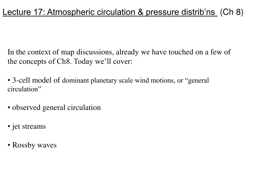
Lecture 17: Atmospheric circulation & pressure distrib’ns (Ch 8) • In the context of map discussions, already we have touched on a few of the concepts of Ch8. Today we’ll cover: • 3-cell model of dominant planetary scale wind motions, or “general circulation” • observed general circulation • jet streams • Rossby waves
We spoke earlier (slide 2, Lec. 9) of the vast and continuous range of scales of motion in the atmosphere… “The largest-scale patterns, called the general circulation, can be considered the background against which unusual events occur, such as” (droughts etc.)… p 213 • Hadley’s (1735) Single-cell Model • ocean-covered planet • sub-solar point perpetually over equator • equatorial heating produces lift and symmetric poleward motion aloft; sink at poles • return equator-ward motion at surface • reasoned earth’s rotation must deflect the wind Fig. 8-2a
Air aloft “diverges” out of the air column, air at surface “converges” into column • Single-cell Model** is • consistent with the observed (and important) surface equatorial “trade winds”, “the most persistent on earth” • though polar surface easterlies emerge only as a long term average, not a prevailing feature • BUT: surface easterlies everywhere would slow down rotation rate of earth! ** Hadley is honoured by a “Hadley Centre for Climate Prediction & Research” in UK Fig. 8-2a
Ferrel’s (1865) Three-cell Model System still conceived as an ocean-covered earth with the subsolar point on the equator • the low lat. “Hadley cell”is thermally • driven by powerful ITCZ convection • the mid lat. Ferrel cell is indirect (forced by the other two) • the high lat. Polar cell is thermally • driven by sink at the poles, • but, we do not get vigorous • overturning • modern view is that only the Hadley • cell is considered “real” Fig. 8-2b
Three-cell Model Equatorial lows + ITCZ Fig. 8-2b
Convective cloud in the ITCZ (“the doldrums”). The ITCZ migrates N-S seasonally with changing solar declination Fig. 8-3
Three-cell model – winds aloft in the Hadley cell Air rising at equator feeds into poleward upper streams, which are deflected by the Coriolis force (to right in N. hemisphere) to produce a zonal component of motion… result: westerly upper currents in both hemispheres About 30o N Rising parcel “meridional” component “zonal” component (of wind velocity) equator Arrows denote rate of movement of the ground surface towards the east… angular mtm of a stationary parcel is largest at the equator Alternative view (Sec. 8-1) each parcel with fixed mass m tends to conserve its “angular momentum” m v r . Constancy of m v r demands an increase of the zonal component (v) of the parcels velocity as it moves north, where the circumference of a latitude line about the earth (2 r ) is shorter. (Friction intervenes so conservation not quite perfect.)
Three-cell Model This poleward moving upper current cools, and around 20-30o latitude (ie. in the “horse latitudes”) it sinks, with consequent adiabatic warming mitigating against cloud at that latitude Fig. 8-2b
Three-cell Model polar surface easterlies do emerge as a long term average Surface westerlies (realistic) + upper easterlies (unrealistic) realistic Fig. 8-2b Land/ocean mix + topography make true climate rather different from 3-cell model
What’s observed: semipermanent surface pressure cells & winds Migrates W and weakens in summer Gone in summer Fig. 8-4a • note strong influence of continents! (Sea-level isobars averaged over 30 Januaries)
What’s observed: mid-tropospheric winds • heights largest over tropics • lowest heights h and strongest gradient h / x (thus, strongest winds) in winter • zonal component generally dominant Fig. 8-6
Polar front jet • Recall P falls more slowly with increasing height in warm air, where density lower • so wherever there are strong horiz temperature gradients (fronts) there are strong • height gradients • strong height gradient implies strong wind perpendicular to the height • gradient (see Geostrophic law)… strongest in winter (stronger T-grdnt) • jet here shown as a climatological feature • as weather feature, irregular - meander & branch Fig. 8-8
L div con con div Waves in mid-latitude mid/upper troposphere causing convergence and divergence aloft... • Long (Planetary/Rossby) Waves — • wavelength 1000’s kilometers • typically 3 - 7 around globe (fewer, longer, stronger in winter) • not always unambiguously identifiable - but can be shown mathematically to exist • in ideal atmos. due to N-S variation of Coriolis force • (usually) move slowly eastward 500 mb
Example of high amplitude Rossby wave over N. America Edmonton low +4oC, high +20oC Winnipeg low -2oC, high +11oC Fig. 8-13 Sept. 22, 1995
Rossby wave moving eastward Fig. 8-12
Rossby wave moving eastward Notice the “short wave” here; covered later – are associated with storms