The Normal Distribution
This presentation delves into the key properties of normal distribution, including its peak location relative to the mean and its symmetric nature. Learn about the significance of the area under the curve, which totals 1, reflecting total probability. We explore variations in normal curves and illustrate how to calculate probabilities using Z-scores. Through a practical example involving sales mileage, we demonstrate how to determine the likelihood of observations falling within specific ranges using standard normal distribution tables or Excel functions.

The Normal Distribution
E N D
Presentation Transcript
The Normal Distribution Prepared by E.G. Gascon
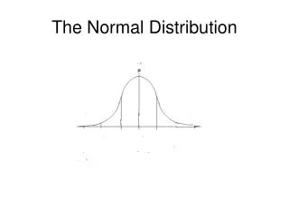
Properties ofNormal Distribution Peak Image text page 487 • It’s peak occurs directly above the mean • The curve is symmetric about the vertical line through the mean. • The curve never touches the x-axis • The area under the curve is always = 1. (This agrees with the fact that the sum of the probabilities in any distribution is 1.)
Variations in Normal Curves One standard deviation is smaller than normal One standard deviation is equal to the normal One standard deviation is larger than normal
The Area Under the Standard Normal Curve 1 standard deviation A B Image from text p 487 • The area of the shaded region under a normal curve form a point A to B is the probability that an observed data value will be between A and B • Between -1 and +1 standard deviations there is 68% of the region, therefore the probability of an observed data value being within 1 standard deviation is 68%, etc.
Problem solved using the Standard Normal Curve The area under a normal curve to the left of x (the data) is the same as the area under the standard normal curve to the left of the z-score for x. What does that mean? The z-score is the formula that converts the raw data (x) from a normal distribution into the lookup values of a STANDARD NORMAL CURVE. [See table in appendix of text or use Excel function =NORMSDIST(Z)] First find the z-score Example: sales force drives an average of 1200 miles, with a standard deviations of 150 miles. 1600 miles is the mileage in question.
What is the probability that a salesperson drives less than 1600 miles? Ans: It is the area to the left of the standard normal curve. Look up 2.67 in the Table of Normal Distributions. There is a 99.62% probability that the salesperson drives less than 1600 miles. 2.67
Using Table of the Normal Distribution Z = 2.67 Table found in text page A-1 back of book Look up 2.6 in the row, and .07 in the column. The intersection is the area to the left, or probability
Or Use Excel function Enter: Results:
What is the probability that a salesperson drives more than 1600 miles? Ans: It is the area to the right of the standard normal curve. Since you know the are to the left of 2.67, the area to the right must be 1 - .9962 = .0038, or .38% probability that a salesperson drives more than 1600 miles. 2.67
What is the probability that a salesperson drives between 1200 and 1600 miles? Ans: The area to the left of 2.67 is already known, it is .9962. It is the difference between driving less than 1600 and less than 1200. 2.67 Find the z value for 1200, , then look it up in the table. Between = .9962 - .5 = .4962 The probability that a salesperson drives between 1200 and 1600 miles is 49.62%
Questions / Comments / Suggestions Please post questions, comments, or suggestions in the main forum regarding this presentation.

