The Normal Distribution
Chapter 9 Probability Distributions. 9.3. The Normal Distribution. MATHPOWER TM 12, WESTERN EDITION. 9.3. 1. Normal Distribution. Many sets of data have common characteristics in how they are distributed. One of the most important probability distributions is the normal distribution.

The Normal Distribution
E N D
Presentation Transcript
Chapter 9 Probability Distributions 9.3 The Normal Distribution MATHPOWERTM 12, WESTERN EDITION 9.3.1
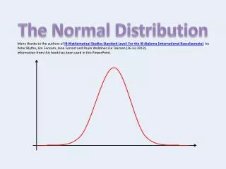
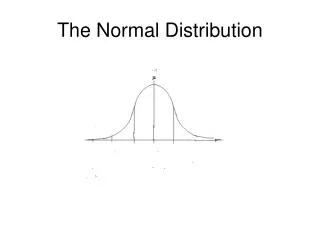
Normal Distribution Many sets of data have common characteristics in how they are distributed. One of the most important probability distributions is the normal distribution. When a set of data forms a bell shape when plotted in a histogram, it is said to be normally distributed. Example: The results of tossing 8 coins 2540 times were recorded and plotted: Frequency 0 1 2 3 4 5 6 7 8 Number of Tails 9.3.2
The Standard Normal Curve One way to analyze a set of data values is to graph its frequency curve. Example: If the frequency of the lifetime of several thousand light bulbs were plotted, the graph would resemble a bell-shaped curve. This bell-shaped curve is the frequency curve of a normal distribution. 9.3.4
The Normal Distribution Curve Basic Properties of the Normal Distribution Curve: 9.3.5
Finding the Area Under the Curve Tables have been developed that correspond to the area under the standard normal curve, N(0, 1). These tables indicate the area under the curve to the left of the z-score. The area under the curve is the region measured from the beginning of the curve to the position of the z-score, relative to the mean. For example: The area for a z-score of -1 is as shown: The area for a z-score of 1 is as shown: 9.3.6
Finding the Area Under the Curve Find the area under the curve for each z-score: go to the tables to find each area and then use a graphing calculator: 1 a) 0.32 1 b) -2.53 Given the area under the curve, find the z-score: go to the tables to find each z-score and then use a graphing calculator: 2 a) 0.0023 2 b) 0.5948 9.3.7
Finding the Area Under the Curve 1. Find the area between z-scores -1.22 and 1.44. The area for z-score is The area for z-score is -1.22 1.44 Therefore, the area between z-scores -1.22 and 1.44 is -1.22 1.44 9.3.9
Finding the Area Under the Curve 2. Find the area between the mean and z-score -1.78. The area for z-score is Therefore, the area between the mean and z-score -1.78 is . 3. Find the area between the mean and z-score 1.78. The area for z-score is Therefore, the area between the mean and z-score 1.78 is 9.3.10
Finding the Area Under the Curve 4. Find the area greater than z-score -0.68. The area for z-score is Therefore, the area between the mean and z-score -0.68 is . 5. Find the area greater than z-score 1.40. The area for z-score is Therefore, the area between the mean and z-score 1.40 is 9.3.11
Finding a Z-Score Given the Area 1. Find the z-score for an area of 0.4901 that is left of the mean. Find the area to the left of the z-score: 2. Find the z-score for an area of 0.2177 greater than the z-score. Find the area to the left of the z-score: 3. Find the z-scores when approximately 80% of the data is evenly distributed about the mean. Find the area to the left of the z-score: 9.3.12
Using Normal Distribution - Applications 1. A television manufacturing company found that the life expectancy of their televisions was normally distributed with a mean of 15 000 h and a standard deviation of 1100 h. a) What percent of the televisions last longer than 17 000 h? b) What percent last between 12 600 h and 16 200 h? c ) In a shipment of 500 televisions, how many would you expect to last less than 13 000 h? a) Calculate the z-score for 17 000 h: 9.3.13
Using Normal Distribution - Applications [cont’d] b) What percent last between 12 600 h and 16 200 h? The area for z-score -2.18 is. The area for z-score 1.09 is Therefore, the area between z-scores -2.18 and 1.09 is Therefore, of the televisions would last between 12 600 h and 16 200 h. 9.3.14
Using Normal Distribution - Applications [cont’d] • In a shipment of 500 televisions, how many • would you expect to last less than 13 000 h? Find the z-scores for 13 000 h: The area for z-score -1.82 is. Therefore, of the televisions would last less than 13 000. Therefore, you would expect televisions to last less than 13 000 h. 9.3.15
Using Normal Distribution - Applications [cont’d] Now, solve the same problem using a graphing calculator: 1. A television manufacturing company found that the life expectancy of their televisions was normally distributed with a mean of 15 000 h and a standard deviation of 1100 h. a) What percent of the televisions last longer than 17 000 h? b) What percent last between 12 600 h and 16 200 h? c ) In a shipment of 500 televisions, how many would you expect to last less than 13 000 h? a) c) b) 9.3.16
Using Normal Distribution - Applications • A staple machine holds 400 staples when loaded. The • mean number of misfires per load is 8 with a standard • deviation of 2.8. Assuming normal distribution, what is the • probability that there will be fewer than 11 but more than 7 misfires per load? Therefore, the probability that there will be fewer than 11 but more than 7 misfires per load is 0.4983. 9.3.17
Using Normal Distribution - Applications 3. A brush manufacturer determines the mean life of his brushes to be five years with a standard deviation of two years. If he guarantees his brushes for three years, what percent of his brushes will he have to replace? Therefore, of the brushes will have to be replaced. 9.3.18
Using Normal Distribution - Applications 4. A manufacturer of calculators finds that the operating lifetime is normally distributed with a mean life of seven years. The manufacturer finds that under a one-year warranty, 4% of the calculators are returned. If 10 000 calculators are manufactured, find the expected number that will last longer than nine years. 9.3.19
Using Normal Distribution - Applications • A steak knife manufacturer guarantees its knives for 12 years and • 3.2% of its knives are returned under warranty. If the standard deviation • is 1.5 years, what is the mean number of years? 9.3.20
Using Normal Distribution - Applications 6. The number of students who scored better than the average and less than a particular z-score is shown below. Find the z-score. 9.3.21
Using Normal Distribution - Applications 7. On a final exam, the mean mark was 68% and the standard deviation was 12%. If John’s mark was 36% and he scored better than five students, how many students wrote the exam? 9.3.22
Using Normal Distribution - Applications • On an exam, the mean mark was 68%, the standard deviation • was 10%, and 40 students had marks between 78% and 82%. • How many students wrote the exam? 9.3.23
Assignment Suggested Questions: A Pages 422 1-13 B Page 423 14-23, 24 ab 9.3.24
Areas Under the Standard Normal Curve, to the Left of z 0.00 0.01 0.02 0.03 0.04 0.05 0.0 0.5000 0.5040 0.5080 0.5120 0.516 0.1 0.5438 0.5478 0.5517 0.5557 0.559 0.2 0.5832 0.5871 0.5910 0.5948 0.5987 0.3 0.6217 0.6255 0.6293 0.6331 0.6368 0.4 0.6591 0.6628 0.6664 0.6700 0.6736 0.5 0.6950 0.6985 0.7019 0.7054 0.7088 0.00 0.01 0.02 0.03 0.04 0.05 -2.9 0.0019 0.0018 0.0018 0.0017 0.0016 -2.8 0.0026 0.0025 0.0024 0.0023 0.0023 -2.7 0.0035 0.0034 0.0033 0.0032 0.0031 -2.6 0.0047 0.0045 0.0044 0.0043 0.0041 -2.5 0.0062 0.0060 0.0057 0.0057 0.0055 Slide 6 Slide 7 9.3.8

