The Normal Distribution
The Normal Distribution. Using Models to Describe Data Distributions. The Density Curve All density curves are based on mathematical models (“equations”) that can be used to describe the frequency for a given datum The area under all densities curves equals 1. the model. the data.

The Normal Distribution
E N D
Presentation Transcript
Using Models to Describe Data Distributions • The Density Curve • All density curves are based on mathematical models (“equations”) that can be used to describe the frequency for a given datum • The area under all densities curves equals 1 the model the data
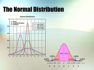
A Very Useful Model • The Normal Distribution is a model that can be used to describe data that is: • Uni-modal • Symmetric • Approximates the “bell curve” • Can be described by the equation:
The “Rule” • Normally distributed data has the following critical property: The 68-95-99.7 Rule
Example… • You have just received the score on your law-school admissions test (LSAT). You got 163. The exam results are normally distributed with N(155,2.6) for that year of testing. In order to apply to a very prestigious law school you must finish in the 97th percentile or better. Can you apply with this score?
Z-Scores and the Standard Normal Distribution • All normal distributions share the same shape • A simple linear transformation can convert any normal distribution to the Standard Form • This gives us the concept of the Z-Score • The 68-95-99.7 rule applies here and can give us a deeper insight into what a z-score means • Converting to Z-scores allows you to use Table A (inside cover of book)
The Standard Normal Distribution • Any normal distribution can be converted to the SND via z-score to N(m,s) N(0,1)
Using z-scores… If the z-score for a data Point is 1 then this means That 84.13% of the samples In the population are less than The value of this data point How do you interpreta z-score of -1.71? Z
Who’s the Greatest? Ty Cobb batted 0.420 In 1911 N(0.266,0.0371) Ted Williams batted 0.406 in 1941 N(0.267,0.0326) z = 4.15 z = 4.26 George Brett batted 0.390 in 1980N(0.261,0.0317) z = 4.07
Normal Quantile Plots (digging deeper) • If you want to use what we have just learned to assess data then you must be sure that the data fits a normal distribution. • Visual inspection (stemplot or histogram is a good start). • The Normal Quantile Plot is even better…Plot data against the probability value that you get for the z-score of the data. If the graph is a straightline the data is normally distributed. Warning! Your text “messed-up!” All of the normal quantile plots have a deceptively labeled x-axis – instead of z-score it should be the probability associated with the z-score.
Example: • Here is the data from an amazing star WZ Sagittae • Am I justified in thinking that the noise in this data is normally distributed? My comparison sources – the “fuzz” in the data is the “noise” or error which I attribute to basic natural processes of measuring light
In conclusion… • Review the summary on pages 83-84. Make sure you understand z-scores, what they mean and how to use them. • Sample problems to gauge your understanding: 1.81, 1.93, 1.97

