Understanding Normal Distribution and Random Variables in Statistics and Probability
This comprehensive guide explores the concepts of random variables and their probability distributions. It distinguishes between discrete and continuous random variables, providing real-world examples for each. The normal distribution, characterized by its bell-shaped curve, is explained along with its significance in statistics. Learn how to calculate z-scores and interpret probabilities using standard normal tables. This resource is essential for anyone looking to grasp the fundamentals of statistical analysis and probability theory.

Understanding Normal Distribution and Random Variables in Statistics and Probability
E N D
Presentation Transcript
(A) Random Variables • Now we wish to combine some basic statistics with some basic probability we are interested in the numbers that are associated with situations resulting from elements of chance i.e. in the values of random variables • We also wish to know the probabilities with which these random variables take in the range of their possible values i.e. their probability distributions
(A) Random Variables Two definitions need to be clarified: • (i) a discrete random variable is a variable quantity which occurs randomly in a given experiment and which can assume certain, well defined values, usually integral examples: number of bicycles sold in a week, number of defective light bulbs in a shipment; discrete random variables involve a count • (ii) a continuous random variable is a variable quantity which occurs randomly in a given experiment and which can assume all possible values within a specified range examples: the heights of men in a basketball league, the volume of rainwater in a water tank in a month; continuous random variables involve a measure
(B) The Normal Distribution • - data obtained by direct measurement (i.e. population heights) is usually continuous rather than discrete (all heights are possible, not just whole numbers) • - continuous data also has statistical distributions and many physical quantities are usually distributed symmetrically and unimodally about the mean statisticians observe this bell shaped curve so often that its model is known as the normal distribution
(B) The Normal Distribution • the graph of the normal distribution is also referred to as the standard normal curve and one defining equation for the curve for our purposes is where z refers to a concept called the z score which takes into account the mean and standard deviation of a set of data: z = (x - )/
we can graph the normal distribution as follows, where the x-axis is the number of standard deviations, , from the mean/median, (the idea behind our z score) the total area under the curve is 1 unit (aising from the fact that the total probability of all outcomes of an event can be at most 1 or 100%) With our z-score, we “set” the mean, , to be 0 and each 1 unit of the x-axis is 1 standard deviation, . (B) The Normal Distribution
to find the area under the curve between any two given z-scores, we can rely on graphs the area under the curve between our two given z-scores means the proportion of values between our two z-scores so if we write p(-2 < z< 1) = 0.81859, we mean that the proportion of data values that are between 2 standard deviation units below the mean and 1 unit above is 0.81859, or as a percentage: 81.859% of our data, or the probability that our data values lie between 2 SD’s below and 1 SD unit above the mean is 0.0.81859 we can illustrate this on a normal distribution graph as follows: (B) The Normal Distribution
(C) The Normal Distribution – Tables of z scores • We can work out the previous example without a graph and shading areas under a graph, by simply using prepared tables: • So to determine the p(-2 < z< 1), we check the table and see that a z value of –2.00 corresponds to a value of 0.0228 this means that the area shaded under the curve, starting from –2.00 all the way left to - is 0.0288 (or 2.88% of the data is more than 2 SD units below the mean) • Likewise, we check the table for our z value of 1.00 and see the value of 0.8413 this means that the area shaded under the curve, starting from 1.00 all the way left to - is 0.8413 (or 84.13% of the data is less than 1 SD units above the mean) • So what do we do with the 2 numbers? Well, we have accounted for some of the data twice the data more than 2 SD units below the mean so this gets subtracted from the first value 0.8413 – 0.0288 = 0.8185 as we saw before with the graph and graphing software
Use the table to evaluate p(z<1.5). Interpret the value. The table gives us the value 0.9332, which means that 93.32% of our data lies 1.5 SD units above the mean and below or the probability of getting a random data point that is at most 1.5 SD units above the mean is 0.9332 We can see this illustrated on the graph (D) Examples
(D) Example Using Standard Normal Tables • For the standard normal variable, find: • (i) p(z < 1) • (ii) p(z < 0.96) • (iii) p(z < 0.03) • Some slightly more challenging examples: • (i) p(z > 1.7) • (ii) p(z < -0.88) • (iii) p(z > -1.53) • And now some in-between values: • (i) p(1.7 < z < 2.5) • (ii) p(-1.12 < z < 0.67) • (iii) p(-2.45 < z < -0.08) • We can also do some inverseproblems • (i) p(z < a) = 0.5478 • (ii) p(z > a) = 0.6 • (iii) p(z < a) = 0.05
(E) Standardizing Normal Distributions • When we have applications wherein we apply a normal distribution (i.e. with any continuous R/V like height, weight of people), each unique application has its own unique mean and standard deviation along with its unique distribution graph • What we wish to accomplish now can we somehow standardize a normal distribution so that one single standardized normal distribution applies for every single possible normal distribution • We can accomplish this by a combination of transformations of our unique data with its unique normal distribution
(E) Standardizing Normal Distributions • So from every data point in our distribution, we will subtract the population’s mean and then divide this difference by the population’s standard deviation we will call this result a “z”-score • So our “formula” for this data transformation is z = (x - )/ • So we then graph the newly transformed data points and we get a standardized normal distribution curve • The two key features on the standardized normal distribution curve are (i) the mean is 0 and (ii) the standard deviation is 1
(G) Working with a Standardized Normal Distribution Ex 1 The heights of all rugby players from India is normally distributed with a mean of 179 cm with a standard deviation of 5 cm. Find the probability that a randomly selected player (i) was less than 181 cm tall (ii) was at least 177.5 cm tall (iii) was between 175 and 190 cm
Solution #1(i) is to use the z-score tables: z = (181-179)/5 = 0.40 So find 0.40 on the tables, which is 0.6554 So given that the table gives us the cumulative area under the curve until the specified z-score (0.40), then we can conclude that 65.5% of the players would be less than 181 cm Alternatively, we can use a GC: We simply select the normalcdf( command and enter the specifics as follows: Normalcdf(-EE99,181,179,5) which tells the GC that you want the heights less than 181 (basically from 181 down to -) and that the population mean is 179 and the SD is 5 Our result is 0.6554 ….. similar to the result from the table (G) Working with a Standardized Normal Distribution
(G) Working with a Standardized Normal Distribution • Solution #1(ii) use the z-score tables however we must realize that the table gives us a cumulative area under the curve up to the given z-score now however we are looking for a value GREATER than the given area • So, using the table, simply find the area under the curve BELOW the given z-score • Then, using the “complement” idea, simply subtract the area from 1 • z-score = (177.5-179)/5 = -0.30 • Table value is 0.4404 (so 44.04% of the area under the curve is to the left of –0.30 on the z-axis) • Therefore, the area representing the probability of our players being GREATER than 177.5 cm would be 1 – 0.4404 = 0.5596 (so this would be the area under the curve, to the right of z = -0.30) • In using the GC, we again simply enter the command normalcdf(177.5, EE99, 179, 5) and get 0.5596 as our answer
(G) Working with a Standardized Normal Distribution • Solution #1(iii) use the z-score tables however we must realize that the table gives us a cumulative area under the curve up to the given z-score now however we are looking for a value BETWEEN 2 given values • So our two z-scores for 175 and 190 are z = –0.80 and z = 2.1, which we can illustrate below
(G) Working with a Standardized Normal Distribution • So, again our tables require several steps in the calculation (i) find the area under the curve that is LESS THAN –0.80 0.2119 (ii) Now find the area under the curve that is less than 2.1 0.9821 Clearly, the 0.9821 total cumulative area includes the 0.2119 that we DO NOT have within our specified range of z-scores (player heights less than 175 cm) Which suggests that we need to subtract the 0.2119 from 0.9821 = 0.7702 • Alternatively, using the GC, we enter normalcdf(175,190,179,5) and get the same 0.7702…..


