Chapter 7 Push and Pull Production Control Systems
Chapter 7 Push and Pull Production Control Systems. Basic Definitions.

Chapter 7 Push and Pull Production Control Systems
E N D
Presentation Transcript
Basic Definitions • MRP. (Materials Requirements Planning). MRP is the basic process of translating a production schedule for an end product (MPS or Master Production Schedule) to a set of requirements for all of the subassemblies and parts needed to make that item. • JIT. Just-in-Time. Derived from the original Japanese Kanban system developed at Toyota. JIT seeks to deliver the right amount of product at the right time. The goal is to reduce WIP (work-in-process) inventories to an absolute minimum.
Why Push and Pull? • MRP is the classic push system. The MRP system computes production schedules for all levels based on forecasts of sales of end items. Once produced, subassemblies are pushed to next level whether needed or not. • JIT is the classic pull system. The basic mechanism is that production at one level only happens when initiated by a request at the higher level. That is, units are pulled through the system by request.
Comparison These methods offer two completely different approaches to basic production planning in a manufacturing environment. Each has advantages over the other, but neither seems to be sufficient on its own. Both have advantages and disadvantages, suggesting that both methods could be useful in the same organization. • Main Advantage of MRP over JIT: MRP takes forecasts for end product demand into account. In an environment in which substantial variation of sales are anticipated (and can be forecasted accurately), MRP has a substantial advantage. • Main Advantage of JIT over MRP: JIT reduces inventories to a minimum. In addition to saving direct inventory carrying costs, there are substantial side benefits, such as improvement in quality and plant efficiency.
MRP Basics • The MRP system starts with the MPS or Master Production Schedule. This is the forecast for the sales of the end item over the planning horizon. The data sources for determining the MPS include: • Firm customer orders • Forecasts of future demand by item • Safety stock requirements • Seasonal variations • Internal orders from other parts of the organization.
The Three Major Control Phases of the Productive System (Fig. 7.2)
The Explosion Calculus • The explosion calculus is a set of rules for converting the master production schedule to a requirements schedule for all subassemblies, components, and raw materials necessary to produce the end item. • There are two basic operations comprising the explosion calculus: • Time phasing. Requirements for lower level items must be shifted backwards by the lead time required to produce the items • Multiplication. A multiplicative factor must be applied when more than one subassembly is required for each higher level item.
The Product Structure Diagram • The product structure diagram is a graphical representation of the relationship between the various levels of the productive system. It incorporates all of the information necessary to implement the explosion calculus. Figure 7-3 (next slide) depicts an end item with two levels of subassemblies.
Explosion Calculus Rules for translating gross requirements at one level to production schedule at that level and requirements at lower levels. Example Basic Equation: Net Req. = Gross req. - Scheduled Receipts - projected on hand inventory Basic Algorithm 1. Compute time-phased requirements 2. Determine Planned Order Release (LS) 3. Compute ending inventory 4. Proceed to next level (if any)
Explosion Calculus Schedule for end item A: Week 8 9 10 11 12 13 14 15 16 17 Gross Req 77 42 38 21 26 112 45 14 76 34 Sch Rpt 12 6 9 Inv 23 Net Req 42 42 32 12 26 112 45 14 76 34 Schedule for item B (1 unit/2 weeks) Week 6 7 8 9 10 11 12 13 14 15 Gross 42 42 32 12 26 112 45 14 76 34 Schedule for item C (2 units/4 weeks) Week 4 5 6 7 8 9 10 11 12 13 Gross 84 84 64 24 52 224 90 28 152 68
Lot Sizing For MRP Systems The simplest lot sizing scheme for MRP systems is lot-for-lot (abbreviated L4L). This means that requirements are met on a period by period basis as they arise in the explosion calculus. However, more cost effective lot sizing plans are possible. These would require knowledge of the cost of setting up for production and the cost of holding each item. This brings to mind the EOQ formula from Chapter 4, which can be used in this context. However, there are better methods.
Statement of the Lot Sizing Problem Assume there is a known set of requirements (r1, r2, . . . rn) over an n period planning horizon. Both the set up cost, K, and the holding cost, h, are given. The objective is to determine production quantities (y1, y2, . . ., yn) to meet the requirements at minimum cost. The feasibility condition to assure there are no stockouts in any period is:
Methods One could apply the EOQ formula by defining but there are better methods. Property of the optimal solution: every optimal solution orders exact requirements: that is, One method that utilizes this property is the Silver Meal Heuristic. The method requires computing the average cost for an order horizon of j periods for j = 1, 2, 3, etc. and stopping at the first instance when the average cost function increases. The average cost for a production quantity spanning j periods, C(j), is given by:
Methods (continued) Another method that is popular in practice is part period balancing. Here one chooses the order horizon to most closely balance the total holding cost with the set-up cost. Finally, a third heuristic is known as the least unit cost heuristic. Here one minimizes the average cost per unit of demand (as opposed to the average cost per period as is done in the Silver Meal heuristic.) The average cost per unit of demand over j periods is given by:
Methods (concluded) • Experimental evidence seems to favor the Silver Meal Heuristic among the four discussed as the most cost efficient. • Optimal lot sizes can be found by using backwards dynamic programming. • A heuristic method for lot sizing subject to capacity constraints is discussed in this section.
Shortcomings of MRP • Uncertainty. MRP ignores demand uncertainty, supply uncertainty, and internal uncertainties that arise in the manufacturing process. • Capacity Planning. Basic MRP does not take capacity constraints into account. • Rolling Horizons. MRP is treated as a static system with a fixed horizon of n periods. The choice of n is arbitrary and can affect the results. • Lead Times Dependent on Lot Sizes. In MRP lead times are assumed fixed, but they clearly depend on the size of the lot required. • Quality Problems. Defective items can destroy the linking of the levels in an MRP system. • Data Integrity. Real MRP systems are big (perhaps more than 20 levels deep) and the integrity of the data can be a serious problem. • Order Pegging. A single component may be used in multiple end items, and each lot must then be pegged to the appropriate item.
Introduction to JIT • JIT (Just In Time) is an outgrowth of the Kanban system developed by Toyota. • Kanban refers to the posting board where the evolution of the manufacturing process would be recorded. • The Kanban system is a manual information system that relies on various types of cards. • It’s development is closely tied to the development of SMED: Single Minute Exchange of Dies, that allowed model changeovers to take place in minutes rather than hours. (The mechanics of a typical Kanban system are pictured in Figure 7-8.)
Kanban System for Two Production Centers (Fig. 7-8)
Features of JIT Systems Small Work-in-Process Inventories. Advantages: 1. Decreases Inventory Costs 2. Improves Production Efficiency 3. Reveals quality problems (see Figure 7-10) Disadvantages: 1. May result in increased worker idle time 2. May result in decreased throughput rate
River/Inventory Analogy Illustrating the Advantages of Just-in-Time
Features of JIT Systems (continued) Kanban Information Flow System Advantages: 1. Efficient tracking of lots 2. Inexpensive implementation of JIT 3. Achieves desired level of WIP Disadvantages: 1. Slow to react to changes in demand 2. Ignores predicted demand patterns
Kanban Information System vs Centralized Information System (MRP)
Features of JIT Systems (continued) JIT Purchasing System Advantages: 1. Inventory reduction 2. Improved coordination 3. Better relationships with vendors Disadvantages: 1. Decreased opportunity for multiple sourcing 2. Suppliers must react quickly 3. Potential for congestion 4. Suppliers must be reliable.
Comparison of MRP and JIT Major study comparing MRP and JIT in practice reveals: • JIT works best in “favorable” manufacturing environments: little demand variability, reliable vendors, and small set up times • MRP (and ROP based on Chapter 5 methods) worked well in favorable environments (comparable to JIT) and better in unfavorable environments.