Push vs. Pull Process Control
Push vs. Pull Process Control. IE 3265 POM Slide Set 9 R. Lindeke, Sp 2005. Basic Definitions.

Push vs. Pull Process Control
E N D
Presentation Transcript
Push vs. Pull Process Control IE 3265 POM Slide Set 9 R. Lindeke, Sp 2005
Basic Definitions • MRP (Materials Requirements Planning). MRP is the basic process of translating a production schedule for an end product (MPS or Master Production Schedule) to a set of time based requirements for all of the subassemblies and parts needed to make that set of finished goods. • JIT Just-in-Time. Derived from the original Japanese Kanban system developed at Toyota. JIT seeks to deliver the right amount of product at the right time. The goal is to reduce WIP (work-in-process) inventories to an absolute minimum.
Why Push and Pull? • MRP is the classic push system. The MRP system computes production schedules for all levels based on forecasts of sales of end items. Once produced, subassemblies are pushed to next level whether needed or not. • JIT is the classic pull system. The basic mechanism is that production at one level only happens when initiated by a request at the higher level. That is, units are pulled through the system by request.
Comparison • These methods offer two completely different approaches to basic production planning in a manufacturing environment. Each has advantages over the other, but neither seems to be sufficient on its own. Both have advantages and disadvantages, suggesting that both methods could be useful in the same organization. • Main Advantage of MRP over JIT: MRP takes forecasts for end product demand into account. In an environment in which substantial variation of sales are anticipated (and can be forecasted accurately), MRP has a substantial advantage. • Main Advantage of JIT over MRP: JIT reduces inventories to a minimum. In addition to saving direct inventory carrying costs, there are substantial side benefits, such as improvement in quality and plant efficiency.
Focusing on JIT • JIT (Just In Time) is an outgrowth of the Kanban system developed by Toyota. • Kanban refers to the posting board (and the inventory control cards posted there) where the evolution of the manufacturing process would be recorded. • The Kanban system is a manual information system that relies on various types of inventory control cards. • It’s development is closely tied to the development of SMED: Single Minute Exchange of Dies, that allowed model changeovers to take place in minutes rather than hours. • The Fundamental Idea of JIT – and Lean Manufacturing Systems in General (an Americanization of the Toyota P. S.) – is to empower the workers to make decisions and eliminate waste wherever it is found
The Tenets of JIT/Lean • Empower the workers: • Workers are our intelligent resources – allow them to exhibit this strength • Workers ultimately control quality lets them do their job correctly (Poka-Yoke) • Don’t pit workers against each other – eliminate “piece-work” disconnected from quality and allow workers to cooperate in teams to design jobs and expectations
The Tenets of JIT/Lean • Eliminate Waste • Waste is anything that takes away from the operations GOAL (to make a profit and stay in business!) • Reduce inventory to only what is absolutely needed • Improve Quality – scrap and rework are costly and disrupt flow • Only make what is ordered • Make setups and changes quickly and efficiently • Employ only the workers needed • Eliminate Clutter – it wastes time
Features of JIT Systems Small Work-in-Process Inventories. Advantages: 1. Decreases Inventory Costs 2. Improves Efficiency 3. Reveals quality problems (see Figure 7-10) Disadvantages: 1. May result in increased worker idle time 2. May result in decreased throughput rate
River/Inventory Analogy Illustrating the Advantages of Just-in-Time Revealing fundamental ‘problems’ is the noted competitive advantages of JIT/Lean
Features of JIT Systems (continued) Kanban Information Flow System Advantages 1. Efficient tracking of lots 2. Inexpensive implementation of JIT 3. Achieves desired level of WIP – based on Number of Kanbans in the system Disadvantages 1. Slow to react to changes in demand 2. Ignores predicted demand patterns (beyond 2 months or so)
Focus on The Kanban • Typically it is a 2-card system • The P (production) Card and W (withdrawal) Card • Limits on product inventory (number of P & W cards) are set by management policy • The count is gradually lowered until problems surface • The actual target level (card count) is based on short term forecasting of demands
Focus on The Kanban – the worker as manager • P cards cycle from their accumulation post at Center 1 to product (when a defined trigger point is reached) and then to output queue • When trigger level is reached, Ct 1 worker pulls product from Ct 1 Wait point queue and replaces the Ct 1 W-cards with Ct 1 P-Cards which then are loaded to the Ct 1 processors – the worker puts Ct 1 W-Cards to his/her acc. Post for W-cards • Finished Product is pushed into the Ct 1 output queue
Focus on The Kanban – the worker as manager • A second worker (Ct 2’s worker) watches for accumulation of Ct 2 W-Cards • When it reaches their trigger level, he/she pulls product into Ct 2 Holding area after replacing Ct 1 P-Cards with their W-Cards – and returns Ct 1 P-Cards to their Acc. Post for Ct. 1 workers benefit • They also watch for accumulation of Ct. 2 P-Cards on their acc. Post and when trigger count is reached they pull product from holding area and replace Ct 2 W-Cards w/ Ct 2 P-Cards then push it into the processors • And around and around they go!
Focus on The Kanban • So how many cards? – speaking of which, a card is associated with a container (lot) of product so the number of P & W cards at a station determines the inventory level of a product!
Focus on The Kanban • Lets look at an example: • 950 units/month (20 productive days) → 48/day • Container size: a = 48/10 = 4.8 → 5 • “L” data: • A. setup is 45 minutes (.75 hour) • B. Setup is 3 minutes (.05 hr) • Wait time: .3 hr/container • Transport time: .45 hr/container • Prod Time: 0.09 hr/each = .45 hr/container
Focus on The Kanban Requires 3*2 = 6*5 = 30 pieces in inventory – also, with 45mins set up 10 times a day means that we consume 450 min or 7.5 hours/day just setting up! Here only 2*2 = 4*5 = 20 pieces and also only .05*10 = 50 min for setup (.833 hr) per day
So, setup reduction impacts Factory Capabilities & Inventory • Lets look at the effect of studies comparing cost of setup vs. inventory cost – like EOQ • Then lets see what we can invest to reduce inventory levels • We will spend money on reducing setup cost (time) and see if reduced inventory will offset our investment • This is the driving force for SMED
Focus on the Penalty Factor • We can effectively model this “a(K)” function as a ‘logarithmic’ investment function • By logarithmic we imply that there is a an increasing cost to continue to reduce setup cost • We state, then, that there is a sum of money that can be invested to yield a fixed percentage of cost reduction • That is (for example) for every investment of $200 the organization can get a 2% reduction in Setup cost
Focus on the Penalty Factor • Lets say that the investment is $ buys a fixed percent reduction in K0 • If we get actually get 10% setup cost reduction for $, then an investment of $ will mean: • Setup cost drops to: 0.9K0 • A second $ investment will lead to a further 10% reduction or: • .9K-.1*.9K = .81K0 • This continues: K3 = .729K0 • Generalizing:
Focus on the Penalty Factor • With that “shape” we can remodel the a(K) logarithmically: • a(K) = b[ln(K0) – ln(K)] • where: • Reverting back to G(Q,K) function – and substituting Q*:
Focus on the Penalty Factor • Finding the K* after the minimization: • To determine what we should do, determine G(K) using K0 and K*
Lets try one: • K0: $1000 • : $95 for each 7.5% reduction in setup cost • Annual quantity: 48000 • Holding cost: $4.50 • MARR is 13%
Continuing: • Investment to get to K* Testing for decision • No investment (K = K0): • At Min K*:
Some terms: • SMED = single minute exchange of dies which means quick tooling change and low setup time (cost) • Inside Processes setup functions that must be done ‘inside’ the machine or done when the machine is stopped • Minimally these would include unbolting departing fixtures/dies and positioning and bolting new fixture/dies to the machine
More Terms: • Outside Setup activities related to tooling changes that can be done ‘outside’ of the machine structure • These would include: • Bringing Tooling to Machine • Bringing Raw Materials to Machine • Getting Prints/QC tools to machine • Etc.
Focus on SMED • When moving from “No Plan” or Step 1 to Step 2 (separating Inside from Outside activities) investments would be relatively low to accomplish a large amount of time (cost) saving • Essentially a new set of change plans and a small amount of training to the Material Handlers so that they are alerted ahead of time and bring the tooling out to the machine before it is needed
Moving to Step 3 and Step 4 • Require investments in Tooling • Require Design Changes • Require Family tooling and adaptors • Require common bolstering attachments • In general requiring larger and larger investments in hardware to achieve smaller and smaller time (cost) savings in setup
Therefore, we can say SMED is: In reality the essence of a Logarithmic setup reduction plan!
Lets Look into Line Balancing • This is a process to optimize the assignment of individual tasks in a process based on a planed throughput of a manufacturing system • It begins with the calculation of a system “Takt” or Cycle time to build the required number of units required over time • From takt time and a structured sequential analysis of the time and steps required to manufacture (assembly) a product, compute the number of stations required on the line • Once station count is determined, assign feasible tasks to stations one-at-a-time filling up to takt time for each station using rational decision/assignment rules
Line Balancing • Feasible tasks are ones that have all predecessors completed (or no predecessors) and take less time that the remaining time at a station • Feasibility is also subject to physical constraints: • Zone Restriction – the task are physically separated taking to much movement time to accomplish both within cycle (like attaching tires to front/back axles on a bus!) • Incompatible tasks – the Grinding/Gluing constraint
Some of the Calculations: • Takt (Cycle) Time: • Minimum # Workstations req’r:
Lets Try One: Times: A 25s; B 33s;C 33s; D 21s; E 40s; F40s; G 44s; H 19s A B C Production Requirement is 400/shift G H D E F
To Perform Assignment we need Assignment Rules: • Primary Rule: • Assign task by order of those having largest number of followers • Secondary Rule: • Assign by longest task time
The Line Balance A B C WS 5 WS 3 G H WS 1 WS 6 D E F WS 2 WS 4
Dealing with Efficiencies • We investigate other Rules – application to improve layout • 1st by followers then by longest time then most followers • Alternating! • Consider line duplication (if not too expensive!) which lowers demand on a line and increases Takt time • The problem of a long individual task • In Koeln, long time stations were duplicated – then the system automatically alternated assignment between these stations