Download
1 / 29
290 likes | 447 Vues
WSN-05 TOULOUSE, Sept. 2005. Fog prediction in a 3D model with parameterized microphysics. Mathias D. Müller 1 , Matthieu Masbou 2 , Andreas Bott 2 , Zavisa I. Janjic 3. 1) Institute of Meteorology Climatology & Remote Sensing University of Basel, Switzerland

E N D
WSN-05 TOULOUSE, Sept. 2005 Fog prediction in a 3D model with parameterized microphysics Mathias D. Müller1, Matthieu Masbou2, Andreas Bott2, Zavisa I. Janjic3 1) Institute of Meteorology Climatology & Remote Sensing University of Basel, Switzerland 2) Meteorological Institue, University of Bonn 3) NOAA/NCEP
NMM_PAFOG Janjic, Z. I., 2003: A Nonhydrostatic Model Based on a New Approach. Meteorology and Atmospheric Physics, 82, 271-285. Droplet number concentration Liquid water content NMM (Nonhydrostatic Mesoscale Model) dynamical framework PAFOG microphysics Condensation/evaporation in the lowest 1500 m is replaced by PAFOG
PAFOG microphysics Detailed condensation/evaporation (parameterized Köhler [Sakakibara 1979, Chaumerilac et. al. 1987]) Evolving droplet population (prognostic mean diameter) Droplet size dependent sedimentation Positive definite advection scheme (Bott 1989)
PAFOG microphysics Supersat. where S is the Supersaturation Assumption on the droplet size distribution : Log-normal function D droplet Diameter Dc,0 mean value of D σc Standart deviation of the given droplet size distribution (σc=0.2)
Boundary conditions for dNc HEIGHT PAFOG TOP 1000 m σc 1000m PAFOG TOP
Nesting GFS NMM-22 NMM_PAFOG GRID: 50 x 50 x 45 (+11 soil layers) dx: 1 km dt: 2s (dynamics) / 10s (physics) CPU: 40 min/24hr on 9 Pentium-4 (very efficient!) NMM_PAFOG NMM-4 NMM-2 15 UTC
19:00 MEZ (3 hr forecast) DROPLET NUMBER CONCENTRATION LIQUID WATER CONTENT PAFOG STANDARD 27 Nov 2004
22:00 MEZ (6 hr forecast) DROPLET NUMBER CONCENTRATION LIQUID WATER CONTENT PAFOG STANDARD 27 Nov 2004
02:00 MEZ (10 hr forecast) DROPLET NUMBER CONCENTRATION LIQUID WATER CONTENT PAFOG STANDARD Accurate sedimentation in PAFOG due to dNc computation. 28 Nov 2004
08:00 MEZ (16 hr forecast) DROPLET NUMBER CONCENTRATION LIQUID WATER CONTENT PAFOG STANDARD 28 Nov 2004
10:00 MEZ (18 hr forecast) DROPLET NUMBER CONCENTRATION LIQUID WATER CONTENT PAFOG STANDARD 28 Nov 2004
qc at 5m height (01:00 MEZ) PAFOG STANDARD
qc at 5m height (06:00 MEZ) PAFOG STANDARD
Cold bias problem Z.Janjic
1D Ensemble prediction system Obser - vations 3D-Model runs 1D-models aLMo NMM-2 Fog forecast period B-matrices variational assimilation PAFOG post-processing COBEL-NOAH NMM-22 NMM-4 www.meteoblue.ch 3D - Forecast time
With assimilation – CASE 1 15:00 observed fog 27-28 Nov 2004
With assimilation – CASE 2 15:00 28-29 Nov 2004
Conclusions 3D model with detailed microphysics Promising first results Computationally very efficient and feasible in todays operational framework More cases and ‘verification’ needed Solves advection problem of 1D approach
GRID of NMM_PAFOG 50 x 50 x 45 27 layers in the lowest 1000 m 11 soil layers Thickness(cm): 0.5 0.75 1.2 1.8 2.7 4.0 6.0 10 30 60 100
Advection statistics Deviation often stronger than signal 1 December 2004 – 30 April 2005, all forecasthours and levels
Fog case - Observations CASE 1 CASE 2
Assimilation example 21 hour forecast of NMM-2 28 Nov 2004 Zürich Kloten Airport
References Berry, E.X & Pranger, M. P. (1974), Equation for calculating the terminal velocities of water drops, J. Appl. Meteor.13, 108-113. Bott, A. (1989), A positive definite advection schemme obtained by nonlinear renormalization of the advective fluxes, Monthly Weather Review117, 1006-1015. Bott, A. & Trautmann, T. (2002), PAFOG – a new efficient forecast model of radiation fog and low-level stratiform clouds, Atmospheric Research64, 191-203. Chaumerliac, N., Richard, E. & Pinty, J.-P. (1987), Sulfur scavenging in a mesoscale model with quasi-spectral microphysic : Two dimensional results for continental and maritime clouds, J. Geophys. Res.92, 3114- 3126. Janjic, Z. I., 2003: A Nonhydrostatic Model Based on a New Approach. Meteorology and Atmospheric Physics, 82, 271-285. Janjic, Z. I., J. P. Gerrity, Jr. and S. Nickovic, 2001: An Alternative Approach to Nonhydrostatic Modeling. Monthly Weather Review, 129, 1164-1178
References Sakakibara, H. (1979), A scheme for stable numerical computation of the condensation process with large time step, J. Meteorol. Soc. Japan57, 349-353. Twomey, S. (1959), The nuclei of natural cloud formation. Part ii : The supersaturation in natural clouds and the variation of cloud droplet concentration, Geophys. Pura Appl.43, 243-249.
Cost function for variational assimilation (physical space) Write in incremental Form Introduce T and U transform to eliminate B from the cost function (Control variable space)
Error covariance matrix NMC-Method (use 3D models):
NMC estimates of B (winter season) NMM-4 1400 UTC large model and time dependence