D. Excitable Media
Explore the behavior and characteristics of excitable media through demonstrations and simulations involving slime mold, cardiac tissue, cortical tissue, and chemical systems. Learn about circular and spiral waves formation, stimulation relay, and recovery in excitable media.

D. Excitable Media
E N D
Presentation Transcript
Examples of Excitable Media • Slime mold amoebas • Cardiac tissue (& other muscle tissue) • Cortical tissue • Certain chemical systems (e.g., BZ reaction) • Hodgepodge machine
Characteristics ofExcitable Media • Local spread of excitation • for signal propagation • Refractory period • for unidirectional propagation • Decay of signal • avoid saturation of medium
Circular & Spiral Waves Observed in: • Slime mold aggregation • Chemical systems (e.g., BZ reaction) • Neural tissue • Retina of the eye • Heart muscle • Intracellular calcium flows • Mitochondrial activity in oocytes
Cause ofConcentric Circular Waves • Excitability is not enough • But at certain developmental stages, cells can operate as pacemakers • When stimulated by cAMP, they begin emitting regular pulses of cAMP
Spiral Waves • Persistence & propagation of spiral waves explained analytically (Tyson & Murray, 1989) • Rotate around a small core of of non-excitable cells • Propagate at higher frequency than circular • Therefore they dominate circular in collisions • But how do the spirals form initially?
Some Explanationsof Spiral Formation • “the origin of spiral waves remains obscure” (1997) • Traveling wave meets obstacle and is broken • Desynchronization of cells in their developmental path • Random pulse behind advancing wave front
Formation of Double Spiral from Pálsson & Cox (1996)
NetLogo SimulationOf Spiral Formation • Amoebas are immobile at timescale of wave movement • A fraction of patches are inert (grey) • A fraction of patches has initial concentration of cAMP • At each time step: • chemical diffuses • each patch responds to local concentration
Response of Patch if patch is not refractory (brown) then if local chemical > threshold then set refractory period produce pulse of chemical (red) else decrement refractory period degrade chemical in local area
Demonstration of NetLogo Simulation of Spiral Formation Run SlimeSpiral.nlogo
Observations • Excitable media can support circular and spiral waves • Spiral formation can be triggered in a variety of ways • All seem to involve inhomogeneities (broken symmetries): • in space • in time • in activity • Amplification of random fluctuations • Circles & spirals are to be expected
NetLogo Simulation of Streaming Aggregation • chemical diffuses • if cell is refractory (yellow) • then chemical degrades • else (it’s excitable, colored white) • if chemical > movement threshold then take step up chemical gradient • else if chemical > relay threshold then produce more chemical (red) become refractory • else wait
Demonstration of NetLogo Simulation of Streaming Run SlimeStream.nlogo
Excitation variable: Recovery variable: Typical Equations forExcitable Medium(ignoring diffusion)
Fixed Points & Eigenvalues stable fixed point unstable fixed point saddle point real parts of eigenvalues are negative real parts of eigenvalues are positive one positive real & one negative real eigenvalue
FitzHugh-Nagumo Model • A simplified model of action potential generation in neurons • The neuronal membrane is an excitable medium • B is the input bias:
NetLogo Simulation ofExcitable Mediumin 2D Phase Space(EM-Phase-Plane.nlogo)
Type II Model • Soft threshold with critical regime • Bias can destabilize fixed point fig. < Gerstner & Kistler
stable manifold Type I Model
Type I vs. Type II • Continuous vs. threshold behavior of frequency • Slow-spiking vs. fast-spiking neurons fig. < Gerstner & Kistler
Modified Martiel & Goldbeter Model for Dicty Signalling Variables (functions of x, y, t): b = intracellular concentration of cAMP g = extracellular concentration of cAMP • = fraction of receptors in active state
Positive Feedback Loop • Extracellular cAMP increases (g increases) • Rate of synthesis of intracellular cAMP increases (F increases) • Intracellular cAMP increases (b increases) • Rate of secretion of cAMP increases • ( Extracellular cAMP increases) See Equations
Negative Feedback Loop • Extracellular cAMP increases (g increases) • cAMP receptors desensitize (f1 increases, f2 decreases, r decreases) • Rate of synthesis of intracellular cAMP decreases (F decreases) • Intracellular cAMP decreases (b decreases) • Rate of secretion of cAMP decreases • Extracellular cAMP decreases (g decreases) See Equations
Dynamics of Model • Unperturbed cAMP concentration reaches steady state • Small perturbation in extracellular cAMP returns to steady state • Perturbation > threshold large transient in cAMP, then return to steady state • Or oscillation (depending on model parameters)
Additional Bibliography • Kessin, R. H. Dictyostelium: Evolution, Cell Biology, and the Development of Multicellularity. Cambridge, 2001. • Gerhardt, M., Schuster, H., & Tyson, J. J. “A Cellular Automaton Model of Excitable Media Including Curvature and Dispersion,” Science247 (1990): 1563-6. • Tyson, J. J., & Keener, J. P. “Singular Perturbation Theory of Traveling Waves in Excitable Media (A Review),” Physica D32 (1988): 327-61. • Camazine, S., Deneubourg, J.-L., Franks, N. R., Sneyd, J., Theraulaz, G.,& Bonabeau, E. Self-Organization in Biological Systems. Princeton, 2001. • Pálsson, E., & Cox, E. C. “Origin and Evolution of Circular Waves and Spiral in Dictyostelium discoideum Territories,” Proc. Natl. Acad. Sci. USA: 93 (1996): 1151-5. • Solé, R., & Goodwin, B. Signs of Life: How Complexity Pervades Biology. Basic Books, 2000. continue to “Part III”