Beam Sampling for the Infinite Hidden Markov Model
140 likes | 289 Vues
Beam Sampling for the Infinite Hidden Markov Model. by. Jurgen Van Gael, Yunus Saatic, Yee Whye Teh and Zoubin Ghahramani. ( ICML 2008 ). Presented by Lihan He ECE, Duke University Nov 14, 2008. Outline. Introduction Infinite HMM Beam sampler Experimental results Conclusion. 2/14.

Beam Sampling for the Infinite Hidden Markov Model
E N D
Presentation Transcript
Beam Sampling for the Infinite Hidden Markov Model by Jurgen Van Gael, Yunus Saatic, Yee Whye Teh and Zoubin Ghahramani (ICML2008) Presented by Lihan He ECE, Duke University Nov 14, 2008
Outline • Introduction • Infinite HMM • Beam sampler • Experimental results • Conclusion 2/14
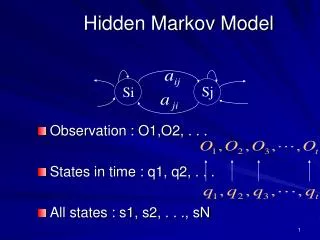
π0 π s0 s1 s2 … sT y1 y2 yT • Model parameters • Hidden state sequence s={s1, s2, …, sT}, • Observation sequence y={y1, y2, …, yT} • π0i = p(s1=i) • πij = p(st=j|st-1=i) Introduction:HMM HMM: hidden Markov model Number of states Complete likelihood 3/14
Introduction:HMM Inference Inference of HMM: forward-backward algorithm • Maximum likelihood: overfitting problem • Bayesian learning: VB or MCMC If we don’t know K a priori • Model selection: inference for all K; computationally expensive. • Nonparametric Bayesian model: iHMM (HMM with an infinite number of states) With iHMM framework • The forward-backward algorithm cannot be applied since the number of states K is infinite. • Gibbs sampling can be used, but convergence is very slow due to the strong dependencies between consecutive time steps. 4/14
Introduction:Beam Sampling Beam sampling = slice sampling + dynamic programming • Slice sampling: limit the number of states considered at each time step to a finite number • Dynamic programming: sample whole state trajectory efficiently Advantages: • Converges in much fewer iterations than Gibbs sampling • Actual complexity per iteration is only marginally more than the Gibbs sampling • Mixes well regardless of strong correlations in the data • More robust with respect to varying initialization and prior distribution 5/14
Infinite HMM Implemented via HDP In the stick-breaking representation Transition probability Emission distribution parameter Infinite hidden Markov model 6/14
Beam Sampler Intuitive thought: only consider the states with large transition probabilities so that the number of possible states in each time step is finite. • Approximation • How to define “large transition probability”? • Might change distributions of other variables Idea: introduce auxiliary variable u such that conditioned on u the number of trajectories with positive probability is finite. • The auxiliary variables do not change the marginal distribution over other variables so MCMC sampling will converge to true posterior 7/14
Only trajectories s with for all t will have non-zero probability given u • Forward filtering: compute • Backward sampling: sample st sequentially for t = T, T-1, …, 2, 1 sequentially for t = 1, 2, …, T Beam Sampler Sampling u: for each t we introduce an auxiliary variable ut with conditional distribution (conditional on π, st-1 and st) Sampling s: we sample the whole trajectory s given u and other variables using a form of forward filtering-backward sampling. 8/14
Beam Sampler Forward filtering • Computing p(st|-) only needs to sum up a finite part of p(st-1|-) • We only need to compute p(st|y1:t , u1:t) for the finitely many st values belonging to some trajectory with positive probability. Backward sampling • Sample sT from • Sample st given the sample for st+1: Sampling φ, π, β: directly from the theory of HDPs 9/14
Experiments Toy example 1: examining convergence speed & sensitivity of prior setting Transition: 1-2-3-4-1-2-3-…, p=0.01 self-transition Observation: discrete HMM: Strong / vague / fixed prior settings for α and γ # states summed up 10/14
Self transition = Experiments Toy example 2: examining performance for positive correlation data 11/14
Experiments Real example 1: changepoint detection (Well data) State partition from one beam sampling iteration Probability that two datapoints are in one segment • Gibbs sampling: • slow convergence • harder decision • Beam sampling: • fast convergence • softer decision 12/14
Experiments Real example 2: text prediction (Alice’s Adventures in Wonderland) • iHMM by Gibbs sampling & beam sampling: • have similar results; • converge to around K=16 states. • VB HMM: • model selection: around K=16 • worse than iHMM 13/14
Conclusion • The beam sampler is introduced for the iHMM inference • Beam sampler combines slice sampling and dynamic programming • Slice sampling limits the number of states considered at each time step to a finite number • Dynamic programming samples whole hidden state trajectories efficiently • Advantages of beam sampler: converges faster than Gibbs sampler mixes well regardless of strong correlations in the data more robust with respect to varying initialization and prior distribution 14/14