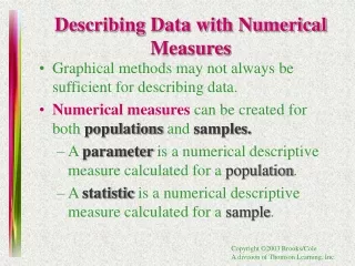
Numerical Measures
Numerical Measures. Numerical Measures. Measures of Central Tendency (Location) Measures of Non Central Location Measure of Variability (Dispersion, Spread) Measures of Shape. Measures of Central Tendency (Location). Mean Median Mode. Central Location. Measures of Non-central Location.

Numerical Measures
E N D
Presentation Transcript
Numerical Measures • Measures of Central Tendency (Location) • Measures of Non Central Location • Measure of Variability (Dispersion, Spread) • Measures of Shape
Measures of Central Tendency (Location) • Mean • Median • Mode Central Location
Measures of Non-central Location • Quartiles, Mid-Hinges • Percentiles Non - Central Location
Measure of Variability (Dispersion, Spread) • Variance, standard deviation • Range • Inter-Quartile Range Variability
Measures of Shape • Skewness • Kurtosis
Summation Notation Let x1, x2, x3, … xn denote a set of n numbers. Then the symbol denotes the sum of these n numbers x1 + x2 + x3 + …+ xn
i 1 2 3 4 5 xi 10 15 21 7 13 Example Let x1, x2, x3, x4, x5 denote a set of 5 denote the set of numbers in the following table.
Then the symbol denotes the sum of these 5 numbers x1 + x2 + x3 + x4 + x5 = 10 + 15 + 21 + 7 + 13 = 66
Final value for i Meaning of parts of summation notation each term of the sum Quantity changing in each term of the sum Starting value for i
i 1 2 3 4 5 xi 10 15 21 7 13 Example Again let x1, x2, x3, x4, x5 denote a set of 5 denote the set of numbers in the following table.
Then the symbol denotes the sum of these 3 numbers = 153 + 213 + 73 = 3375 + 9261 + 343 = 12979
Mean Let x1, x2, x3, … xn denote a set of n numbers. Then the mean of the n numbers is defined as:
i 1 2 3 4 5 xi 10 15 21 7 13 Example Again let x1, x2, x3, x4, x5 denote a set of 5 denote the set of numbers in the following table.
Interpretation of the Mean Let x1, x2, x3, … xn denote a set of n numbers. Then the mean, , is the centre of gravity of those the n numbers. That is if we drew a horizontal line and placed a weight of one at each value of xi , then the balancing point of that system of mass is at the point .
xn x1 x3 x4 x2
In the Example 21 7 10 13 15 20 0 10
The mean, , is also approximately the center of gravity of a histogram
The Median Let x1, x2, x3, … xn denote a set of n numbers. Then the median of the n numbers is defined as the number that splits the numbers into two equal parts. To evaluate the median we arrange the numbers in increasing order.
If the number of observations is odd there will be one observation in the middle. This number is the median. If the number of observations is even there will be two middle observations. The median is the average of these two observations
i 1 2 3 4 5 xi 10 15 21 7 13 Example Again let x1, x2, x3, x3 , x4, x5 denote a set of 5 denote the set of numbers in the following table.
The numbers arranged in order are: 7 10 13 15 21 Unique “Middle” observation – the median
Example 2 Let x1, x2, x3 , x4, x5 , x6 denote the 6 denote numbers: 23 41 12 19 64 8 Arranged in increasing order these observations would be: 8 12 19 23 41 64 Two “Middle” observations
Median = average of two “middle” observations =
Example The data on N = 23 students Variables • Verbal IQ • Math IQ • Initial Reading Achievement Score • Final Reading Achievement Score
Data Set #3 The following table gives data on Verbal IQ, Math IQ, Initial Reading Acheivement Score, and Final Reading Acheivement Score for 23 students who have recently completed a reading improvement program Initial Final Verbal Math Reading Reading Student IQ IQ Acheivement Acheivement 1 86 94 1.1 1.7 2 104 103 1.5 1.7 3 86 92 1.5 1.9 4 105 100 2.0 2.0 5 118 115 1.9 3.5 6 96 102 1.4 2.4 7 90 87 1.5 1.8 8 95 100 1.4 2.0 9 105 96 1.7 1.7 10 84 80 1.6 1.7 11 94 87 1.6 1.7 12 119 116 1.7 3.1 13 82 91 1.2 1.8 14 80 93 1.0 1.7 15 109 124 1.8 2.5 16 111 119 1.4 3.0 17 89 94 1.6 1.8 18 99 117 1.6 2.6 19 94 93 1.4 1.4 20 99 110 1.4 2.0 21 95 97 1.5 1.3 22 102 104 1.7 3.1 23 102 93 1.6 1.9
Computing the Median Stem leaf Diagrams Median = middle observation =12th observation
Some Comments • The mean is the centre of gravity of a set of observations. The balancing point. • The median splits the obsevations equally in two parts of approximately 50%
The median splits the area under a histogram in two parts of 50% • The mean is the balancing point of a histogram 50% 50% median
For symmetric distributions the mean and the median will be approximately the same value 50% 50% Median &
For Positively skewed distributions the mean exceeds the median • For Negatively skewed distributions the median exceeds the mean 50% 50% median
An outlier is a “wild” observation in the data • Outliers occur because • of errors (typographical and computational) • Extreme cases in the population
The mean is altered to a significant degree by the presence of outliers • Outliers have little effect on the value of the median • This is a reason for using the median in place of the mean as a measure of central location • Alternatively the mean is the best measure of central location when the data is Normally distributed (Bell-shaped)
Summarizing Data Graphical Methods
Histogram Grouped Freq Table Stem-Leaf Diagram
Numerical Measures • Measures of Central Tendency (Location) • Measures of Non Central Location • Measure of Variability (Dispersion, Spread) • Measures of Shape The objective is to reduce the data to a small number of values that completely describe the data and certain aspects of the data.
Mean Let x1, x2, x3, … xn denote a set of n numbers. Then the mean of the n numbers is defined as:
Interpretation of the Mean Let x1, x2, x3, … xn denote a set of n numbers. Then the mean, , is the centre of gravity of those the n numbers. That is if we drew a horizontal line and placed a weight of one at each value of xi , then the balancing point of that system of mass is at the point .
xn x1 x3 x4 x2
The mean, , is also approximately the center of gravity of a histogram
The Median Let x1, x2, x3, … xn denote a set of n numbers. Then the median of the n numbers is defined as the number that splits the numbers into two equal parts. To evaluate the median we arrange the numbers in increasing order.
If the number of observations is odd there will be one observation in the middle. This number is the median. If the number of observations is even there will be two middle observations. The median is the average of these two observations
Measures of Non-Central Location • Percentiles • Quartiles (Hinges, Mid-hinges)