Numerical Summary Measures
Numerical Summary Measures. Lecture 03: Measures of Variation and Interpretation, and Measures of Relative Position. Measures of Variation. Consider the following three data sets: Data 1: 1, 2, 3, 4, 5 Data 2: 1, 1, 3, 5, 5 Data 3: 3, 3, 3, 3, 3

Numerical Summary Measures
E N D
Presentation Transcript
Numerical Summary Measures Lecture 03: Measures of Variation and Interpretation, and Measures of Relative Position
Measures of Variation • Consider the following three data sets: • Data 1: 1, 2, 3, 4, 5 • Data 2: 1, 1, 3, 5, 5 • Data 3: 3, 3, 3, 3, 3 • For these data sets, the mean and the median are clearly identical. • But, they are different data sets! • The need to measure the variation in the data.
On the Perils of an “Average Value” • Situation: Man has his head in a very hot compartment, and his feet feeling very cold. • Question: Mr., how are you feeling? • Reply: Oh, on the average, I am just fine! … • Crash! Dead!
Sample Variance • To measure degree of variation, one could look at the values of the deviations of the observations from its sample mean. • The sample variance, denoted by S2, is defined to be the ‘average’ of the squared deviations of the observations from its sample mean.
Computational Formula • Definitional formula not very efficient for purposes of computation of the sample variance. • The computational formula is oftentimes used.
Properties • It has squared units … which leads to defining the standard deviation. • It is always nonnegative, and equals zero if and only if all the observations are identical. • The larger the value, the more variation in the data. • The divisor of (n-1) instead of n makes the sample variance “unbiased” for the population variance (s2) … will be explained when we get into inference.
Standard Deviation • The sample standard deviation, denoted by S, is the positive square root of the sample variance. • Purpose: to have a measure with the same units of measurements as the original observations.
Illustration of Computation • Data set in the example for the mean and median. • Data: 122, 135, 110, 126, 100, 110, 110, 126, 94, 124, 108, 110, 92, 98, 118, 110, 102, 108, 126, 104, 110, 120, 110, 118, 100, 110, 120, 100, 120, 92 • We illustrate computations using the definitional and computational formulas in a spreadsheet-type format.
Example … continued • The spreadsheet-type table on the next slide is obtained from an Excel worksheet. • The first three columns illustrates the computation using the definitional formula. • The last column is used to illustrate the computation using the computational formula. • Details will be provided in class!
Explanations of Columns in the Sheet • Column 1: contains the values of X, Sum of X, and Sample Mean. • Column 2: contains the deviations, Dev = X-SampleMean, and the Sum of Deviations. • Column 3: contains the squared deviations, Sum of squared deviations, variance, and the standard deviation (via definitional formula). • Column 4: contains the squared X; sum of squared X, and the variance (via the computational formula).
Population Parameters (Analogs) • If the quantities are computed from the population values, then we obtain population parameters such as the mean, variance and standard deviations. • The notation are as follows:
Information from Mean and Standard Deviation • Empirical Rule: For symmetric mound-shaped distributions: • Percentage of all observations within 1 standard deviation of the mean is approximately 68%. • Percentage of all observations within 2 standard deviations of the mean is approximately 95%. • Percentage of all observations within 3 standard deviations of the mean is approximately 100%. • Thus, usually no observations will be more than 3 standard deviations of the mean!
Information … continued • Chebyshev’s Rule: For any distribution (be it symmetric, skewed, bi-modal, etc.), we always have that: • Percentage of all observations within 1 standard deviation of the mean is at least 0%. • Percentage of all observations within 2 standard deviations of the mean is at least 75%. • Percentage of all observations within 3 standard deviations of the mean is at least 88.89%. • More generally, the percentage of observations within k standard deviations of the mean is at least (1 - 1/k2).
Illustration of these Rules • Consider the sample data with 30 observations considered earlier. • Data: 122, 135, 110, 126, 100, 110, 110, 126, 94, 124, 108, 110, 92, 98, 118, 110, 102, 108, 126, 104, 110, 120, 110, 118, 100, 110, 120, 100, 120, 92 • Recall that: • Sample mean = 111.1 • Sample standard deviation = 11.11 • Percentages in the intervals of form: • [Mean - kS, Mean + kS]
Measure of Relative Standing: Z-Score Given a data set, the z-score, called the standardized score, associated with an observation whose value is x is given by It measures the distance of x from the sample mean in terms of the number of standard deviations. A negative (positive) value indicates the value x is smaller (larger) than the sample mean.
Percentiles • Given a set of n observations, the 100pth percentile, where 0 < p < 1, is that value which is larger than 100p% of all the observation, and less than 100(1-p)% of the observations. • For example, the 95th percentile is the value larger than 95% of all the observations and it is smaller than 5% of all the observations.
Measures of Relative Standing: Quartiles • The first quartile, denoted by Q1, is the 25th percentile of the data set. • The third quartile, denoted by Q3, is the 75th percentile of the data set. • The second quartile, which is the 50th percentile, is simply the median of the data set, M.
Computing the Quartiles • Divide the arranged data set into two parts using the median as cut-off. • If the sample size n is odd, then the median should be included in each group; while if n is even then the median is not included in either group. • First quartile (Q1) is the median of the lower group. • Third quartile (Q3) is the median of the upper group.
Example: Quartile Computation • Arranged Data: • 92, 92, 94, 98, 100, 100, 100, 102, 104, 108, 108, 110, 110, 110, 110, 110, 110, 110, 110, 118, 118, 120, 120, 120, 122, 124, 126, 126, 126, 135 • M = 110 = average of 15th and 16th values. • Q1 = in 8th position = 102 • Q3 = in 23rd position = 120.
Box Plots • Another graphical summary of the data is provided by the boxplot. This provides information about the presence of outliers. • Steps in constructing a boxplot are as follows: • Calculate M, Q1, Q3, and the minimum and maximum values. • Form a box with left and right ends being at Q1 and Q3, respectively. • Draw a vertical line in the box at the location of the median. • Connect the min and max values to the box by lines.
The BoxPlot • For the systolic blood pressure data set, the resulting boxplot, obtained using Minitab, is shown below. HV Q3 M Q1 LV
Comparative BoxPlots The boxplot could also be used to make a comparison of the distributions of different groups. This could be achieved by presenting the boxplots of the different groups in a side-by-side manner. We demonstrate this idea using the Beanie Babies Data on page 91. This data set contains the following variable: Name: name of beanie baby Age: in months, since 9/98 Status: R=retired, C=current Value: Value of baby
Comparative BoxPlots of Value by Status Distributions for both groups very right-skewed!