Download
1 / 29
290 likes | 422 Vues
Erosion rate formulation and modeling of turbidity current. Ao Yi and Jasim Imran Department of Civil and Environmental Engineering. Recent Progress in numerical modeling of density currents considering the vertical structure.

E N D
Erosion rate formulation and modeling of turbidity current Ao Yi and Jasim Imran Department of Civil and Environmental Engineering
Recent Progress in numerical modeling of density currents considering the vertical structure • Stacey & Bowen (1988): Temporal evolution of vertical structure of density and turbidity current using zero Equation turbulence model. Convective and diffusive terms in the flow direction neglected. • Meiburg et al. : (2000) Used DNS to solve the Navier Stokes equations for density current at low Reynolds number (with Boussinesq assumption) • Imran, Kassem, & Khan AND Kassem & Imran (2005): Used the commercial flow solver FLUENT to simulate density current in confined and unconfined straight and sinuous channel. The model used RANS Equations and k-e turbulence closure • Felix (2001): Solved the RANS equations for lock exchange particulate currents at large scale using 2 equation Mellor-Yamada level 2.5 model • Choi and García (2002): Simulated continuous dilute saline density current on a ramp by solving 2-D steady state boundary layer equation using the 2 equation k-epsilon turbulence model • Huang, Imran & Pirmez (2005): Solved 2 equation k-epsilon model for turbidity current for well-sorted sediment. Considered bed level change by adjusting the bed boundary and the grids during the computation. Successfully reproduced Garcia’s (1990) experiment including the flow structure and bed level changes.
For conservative density currents, numerical modeling has certainly reached very high level of sophistication. Where are we in terms of modeling turbidity currents and the morphological changes at the field scale ? Does not matter how much detail of the current one can churn out from the most sophisticated solution of the Navier-Stoke Equations, there is no escape from van Rijn or Akiyama-Fukushima, or Garcia-Parker or Smith-McLean or some other ‘empirical relationship’ that defines sediment entrainment from the bed!
Suppose we make numerical model runs keeping the boundary conditions and computational grid same but choose different entrainment relationships in different runs Can we expect to see the same result?
We need to pay serious attention to • the modeling of turbulent kinetic energy (TKE) & • the sediment entrainment from the bed
Peak velocity region poses a strong barrier to mixing If there is a sediment pick up, can The particles diffuse above the ‘fish-trap’? Barrier to diffusion
Consider three different closure models • k – l model ( 1 eqn model) Turbulence kinetic energy (k) is calculated using transport equation where turbulence length scale (l) is calculated using an empirical formula. • q2– l model ( 1 eqn model) Turbulence velocity scale (q) is calculated using transport equation where turbulence length scale (l) is calculated using an empirical formula. • k – ε model ( 2 eqn model) Both turbulence kinetic energy (k) and its dissipation rate (ε) are calculated using transport equations.
Three erosion rate relationships 1. Akiyama and Fukushima (1985) –E-I
What is ignition condition? For known values of current thickness, sediment size, and bed slope, there is a combination of velocity, turbulent kinetic energy, and concentration at which the flow will ignite or become erosional.
Set the left side of these equations equal to zero and find solution for U,Y, and KPick the lowest positive value
E-II-I E-III-I E-III-II
UI vs. h0/Ds for Ds = 0.03 mm, 0.06 mm, and 0.1 mm. S and Cf* are respectively set equal to 0.05 and 0.004
Phase diagram computed for the case: Ds = 0.1 mm, h0 = 5 m, Cf* = 0.004 and S = 0.1.A-U0 = 0.6 m/s, 0 = 2.0×10⁻⁴ m 2 /s, and K0 = 8.0×10⁻³ m 2/s 2
Phase diagram computed for the case: Ds = 0.03 mm, h0 = 1 m, Cf* = 0.004 and S = 0.05. C-U0 = 0.2 m/s, 0 = 2.0×10⁻⁵ m 2/s, and K0 = 1.0×10⁻³ m 2/s 2
Cross field for case Ds = 0.1 mm, h0 = 5 m, Cf* = 0.004, and S = 0.1
Cross field for case Ds = 0.03 mm, h0 = 1 m, Cf* = 0.004, and S = 0.05
Conclusions • 1. The ignition values obtained with different models can vary widely. • 2. A turbidity current predicted to be subsiding by one entrainment relation could turn out to be igniting when a different entrainment model is used. • 3. Important implication in the numerical modeling of turbidity current • 4. Further research on the topic of sediment entrainment is crucial
ACKNOWLEDGMENT Funding from the National Science Foundation (OCE-0134167) is gratefully acknowledged.