Download
1 / 37

E N D
5. Empirical Orthogonal Functions The purpose is to discuss Empirical Orthogonal Functions (EOF), both in method and application. When dealing with teleconnections in the previous chapter we came very close to EOF, so it will be a natural extension of that theme. However, EOF opens the way to an alternative point of view about space-time relationships, especially correlation across distant times as in analogues. EOFs have been treated in book size texts, most recently in Jolliffe (2002), a principal older reference being Preisendorfer(1988). The subject is extremely interdisciplinary, and each field has its own nomenclature, habits and notation. Jolliffe’s book is probably the best attempt to unify various fields. The term EOF appeared first in meteorology in Lorenz(1956). Zwiers and von Storch(1999) and Wilks(1995) devote lengthy single chapters to the topic. Here we will only briefly treat EOF or PCA (Principal Component Analysis) as it is called in most fields. Specifically we discuss how to set up the covariance matrix, how to calculate the EOF, what are their properties, advantages, disadvantages etc. We will do this in both space-time set-ups already alluded to in Eqs (2.14) and (2.14a). There are no concrete rules as to how one constructs the covariance matrix. Hence there are in the literature matrices based on correlation, based on covariance etc. Here we follow the conventions laid out in Chapter 2. The postprocessing and display conventions of EOFs can also be quite confusing. Examples will be shown, for both daily and seasonal mean data, for both the Northern and Southern Hemisphere.
5.1 Methods and definitions 5.1.1 Working definition: Here we cite Jolliffe (2002, p 1). “The central idea of principal component analysis (PCA) is to reduce the dimensionality of a data set consisting of a large number of interrelated variables, while retaining as much as possible of the variation present in the data set. This is achieved by transforming to a new set of variables, the principle components, which are uncorrelated, and which are ordered so that the first few retain most of the variation present in all of the original variables.” The italics are Jolliffe’s. PCA and EOF analysis is the same.
5.1.2 The Covariance Matrix One might say we traditionally looked upon a data set f(s,t) as a collection of time series of length nt at each of nslocations. In Chapter 2 we described that after taking out a suitable reference { } from a data set f(s,t), usually the space dependent time-mean (or ‘climatology’), the covariance matrix Q can be formed with elements as given by (2.14): qij = ∑ f (si, t) f (sj , t) / nt t where si and sj are the i-thand j-thpoint (gridpoint or station) in space. The matrix Q is square, has dimension ns, is symmetric and consists of real numbers. The average of all qii (the main diagonal) equals the space time variance (STV) as given in (2.16). The elements of Q have great appeal to a meteorological audience. Fig.4.1 featured two columns of the correlation version of Q in map form, the NAO and PNA spatial patterns, while Namias(1981) published all columns of Q (for seasonal mean 700 mb height data) in map form in an atlas.
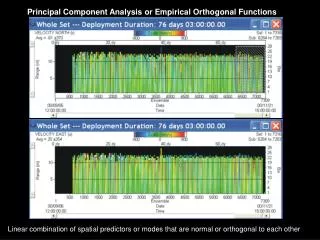
5.1.3. The Alternative Covariance Matrix One might say with equal justification that we look upon f(s,t) alternatively as a collection of nt maps of size ns. The alternative covariance matrix Qa contains the covariance in space between two times ti and tj given as in (2.14a): qaij = ∑ f (s, ti ) f (s, tj ) / ns s where the superscript a stands for alternative. Qa is square, symmetric and consists of real numbers, but the dimension is nt by nt , which frequently is much less than ns by ns , the dimension of Q. As long as the same reference {f} is removed from f(s,t) the average of the qaii over all i, i.e. the average of main diagonal elements of Qa, equals the space-time variance given in (2.16). The average of the main diagonal elements of Qa and Q are thus the same. The elements of Qa have apparently less appeal than those of Q (seen as PNA and NAO in Fig.4.1). It is only in such contexts as in ‘analogues’, see Chapter 7, that the elements of Qa have a clear interpretation. The qaij describe how (dis)similar two maps at times ti and tj are.
When we talk throughout this text about reversing the role of time and space we mean using Qa instead of Q. The use of Q is more standard for explanatory purposes in most textbooks, while the use of Qa is more implicit, or altogether invisible. For understanding it is important to see the EOF process both ways.
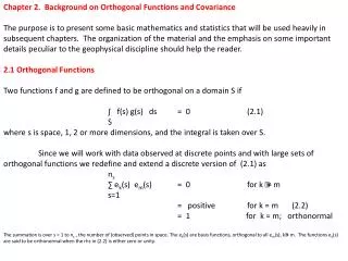
5.1.4 The covariance matrix: context The covariance matrix typically occurs in a multiple linear regression problem where f (s,t) are thepredictors, and y(t) is a dummy predictand, 1 <= t <= nt. Here we first follow Wilks(1995; p368-369). A ‘forecast’ of y (denoted as y*) is sought as follows: y*(t) = ∑ f (s, t) b (s) + constant, (5.1) s where b(s) is the set of weights to be determined. As long as the time mean of f was removed, the constant is zero. The residual U = ∑ { y (t) - y*(t) }2 needs to be minimized. t ∂ U / ∂ b(s) = 0 leads to the “normal” equations, see Eq 9.23 in Wilks(1995), given by: Q b = a, where Q is the covariance matrix and a and b are vectors of size ns. The elements of vector a consist of ∑ f (t , si) y(t) / nt. Since Q and a are known, b can be solved for, in principle. t --- continued ----
5.1.4 The covariance matrix: context continued Note that Q is the same for any y. (Hence y is a ‘dummy’.) The above can be repeated alternatively for a dummy y(s) y*(s) = ∑ f(s, t) b(t) (5.1a) where the elements of b are a function of time. This leads straightforwardly to matrix Qa. (5.1a) will also be the formal approach to constructed analogue, see chapter 7. Q and Qa occur in a wide range of linear prediction problems and Q and Qa depend only on f(s,t), here designated as the predictor data set. In the context of linear regression it is an advantage to have orthogonal predictors, because one can add one predictor after another and add information (variance) without overlap, i.e. new information not accounted for by other predictors. In such cases there is no need for backward/forward regression and one can reduce the total number of predictors in some rational way. We are thus interested in diagonalized versions of Q and Qa (and the linear transforms of f(s,t) underlying the diagonalizedversion of the two Qs).
5.1.5 EOF calculated through eigen-analysis of cov matrix In general a set of observed f(s,t) are not orthogonal, i.e. ∑ f (si, t) f (sj , t) and ∑ f (s, ti ) f (s, tj) are not zero for i ≠ j. Put another way: neither Q nor Qa are diagonal. Here some basic linear algebra can be called upon to diagonalize these matrices and transform the f (s,t) to become a set of uncorrelated or orthogonal predictors. For a square, symmetric and real matrix, like Q or Qa, this can be done easily, an important property of such matrices being that all eigenvalues are real and positive and the eigenvectors are orthogonal. The classical eigenproblem for matrix B can be stated: B em = λmem (5.2) where e is the eigenvector and λis the eigenvalue, and for this discussion B is either Q or Qa. The index m indicates there is a set of eigenvalues and vectors. Notice the non-uniqueness of (5.2) - any multiplication of em by a positive or negative constant still satisfies (5.2). Often it will be convenient to assume that the norm |e| is 1 for each m.
Any symmetric real matrix B has these properties: 1) The em’s are orthogonal 2) E-1 B E, where matrix E contains all em , results in a matrix Γwith the elements λmat the main diagonal, and all other elements zero. This is one obvious recipe to diagonalize B (but not the only recipe!). 3) all λm> 0, m=1, ...M. Because of property 1 the em(s) are a basis, orthogonal in space, which can be used to express: f ( s, t) = αm(t)em(s) (5.3) where the αm(t) are calculated, or thought of, as projection coefficients, see Eq (2.6). But the αm(t) are orthogonal by virtue of property #2. It is actually only the 2nd step/property that is needed to construct orthogonal predictors in the context of Q. Here we thus have the very remarkable property of bi-orthogonality of EOFs - both αm(t) and em(s) are an orthogonal set. With justification the αm(t) can be looked upon as basis functions also, and (5.3) is also satisfied when the em(s) are calculated by projecting the data onto αm(t).
We can diagonalizeQa in the same way, by calculating its eigenvectors. Now the transformed maps (linear combinations of original maps) become orthogonal due to step 2, and the transformed time series are a basis because of property 1. (Notation may be a bit confusing here, since, except for constants, the e’s will be α’s and vice versa, when using Qa instead of Q.) One may write: Q em = λmem (5.2) Qaema = λmaema (5.2a) such that the e’s are calculated as eigenvectors of Qa or Q. We then have f ( s, t) = ∑ αm(t) em(s) (5.3) f ( s, t) = ∑ ema(t) βm(s) (5.3a) where the α’s and β’s are obtained by projection, and the e’s are obtained as eigenvector. When ordered by EV, λm= λma, and except for multiplicative constants βm(s)=em(s) and αm(t)=ema(t), so (5.3) alone suffices to describe EOF. Note that αm(t) and em(s) cannot both be normed at the same time while satisfying (5.3). This causes considerably confusion. In fact all one can reasonably expect is: f ( s, t) = ∑ αm(t)/c em(s)*c (5.3b) where c is a constant (positive or negative). (5.3b) is consistent with both (5.3) and (5.3a). Neither the polarity, nor the norm is settled in an EOF procedure. The only unique parameter is λm. Since there is only one set of bi-orthogonal functions, it follows that during the above procedure Q and Qa are simultaneously diagonalized, one explicitly, the other implicitly for free. It is thus advantageous in terms of computing time to choose the covariance matrix with the smallest dimension. Often, in meteorology nt<< ns. Savings in computer time can be enormous.
5.1.6 Explained variance EV The eigenvalues can be ordered: λ1> λ2> λ3..... > λM> 0. Moreover: M ns ∑ λm= ∑ qii/ns = STV m=1 i=1 The λm are thus a spectrum, descending by construction, and the sum of the eigenvalues equals the space time variance. Likewise M M ∑ λm = ∑ qakk /nt = STV m=1 k=1 The eigenvalues for Q and Qa are the same and have the units of variance. The total number of eigenvalues, M, is at most the smaller of ns and nt In the context of Q one can also write: explained variance of mode m (λm) = ∑ α2m(t) /nt as long as |e|=1. Jargon: mode m ‘explains’ λmof STV or λm /∑ λm *100. % EV 5.2 Examples next
Fig.5.1 Display of four leading EOFs for seasonal (JFM) mean 500 mb height. Shown are the maps and the time series. A postprocessing is applied, see Appendix I, such that the physical units (gpm) are in the time series, and the maps have norm=1. Contours every 0.2, starting contours +/- 0.1. Data source: NCEP Global Reanalysis. Period 1948-2005. Domain 20N-90N
Fig.5.2. Same as Fig 5.1, but now daily data for all Decembers, Januaries and Februaries during 1998-2002.
Fig.5.4 Display of four leading alternative EOT for seasonal (JFM) mean 500 mb height. Shown are the regression coefficient between the basepoint in time (1989 etc) and all other years (timeseries) and the maps of 500mb height anomaly (geopotential meters) observed in 1989, 1955 etc . In the upper left for raw data, in the upper right after removal of the first EOT mode, lower left after removal of the first two modes. A postprocessing is applied, see Appendix I, such that the physical units (gpm) are in the time series, and the maps have norm=1. Contours every 0.2, starting contours +/- 0.1. Data source: NCEP Global Reanalysis. Period 1948-2005. Domain 20N-90N
Fig.5.5, the same as Fig 5.1, but obtained by starting the iteration method (see Appendix II) from alternative EOTs, instead of regular EOT. Compared to Fig.5.1 only the polarity may have changed.
Fig.5.1 Display of four leading EOFs for seasonal (JFM) mean 500 mb height. Shown are the maps and the time series. A postprocessing is applied, see Appendix I, such that the physical units (gpm) are in the time series, and the maps have norm=1. Contours every 0.2, starting contours +/- 0.1. Data source: NCEP Global Reanalysis. Period 1948-2005. Domain 20N-90N
EOT-normal Q is diagonalized Qa is not diagonalized (1) is satisfied with αm orthogonal Q tells about Teleconnections Matrix Q with elements: qij=∑ f(si,t)f(sj,t) t iteration Rotation EOF Both Q and Qa Diagonalized (1) satisfied – Both αm and em orthogonal αm (em) is eigenvector of Qa(Q) Laudable goal: f(s,t)=∑ αm(t)em(s) (1) m Discrete Data set f(s,t) 1 ≤ t ≤ nt ; 1 ≤ s ≤ ns iteration Arbitrary state Rotation iteration Matrix Qa with elements: qija=∑f(s,ti)f(s,tj) s EOT-alternative Q is not diagonalized Qa is diagonalized (1) is satisfied with em orthogonal Qa tells about Analogues Fig.5.6: Summary of EOT/F procedures.
Fig 5.7. Explained Variance (EV) as a function of mode (m=1,25) for seasonal mean (JFM) Z500, 20N-90N, 1948-2005. Shown are both EV(m) (scale on the left, triangles) and cumulative EV(m) (scale on the right, squares). Red lines are for EOF, and blue and green for EOT and alternative EOT respectively.
Fig.5.8 Display of four leading EOFs for seasonal (OND) mean SST. Shown are the maps on the left and the time series on the right. Contours every 1C, and a color scheme as indicated by the bar. Data source: NCEP Global Reanalysis. Period 1948-2004. Domain 45S-45N
Fig.5.9 Display of four leading EOFs for seasonal (JFM) mean 500 mb streamfunction. Shown are the maps and the time series. A postprocessing is applied, see Appendix I, such that the physical units (m*m/s) are in the time series, and the maps have norm=1. Contours every 0.2, starting contours +/- 0.1. Data source: NCEP Global Reanalysis. Period 1948-2005. Domain 20N-90N
simplifications • Why simplify? • Rotated EOF • EOT, EOT-alternative • Surgical patches.
Other • Complex EOF • Extended or joint EOF • Cross-data-sets empirical orthogonal …., come listen April 23.
Common misunderstandings • EOF are eigen vectors • EOF can only do standing patterns • The 1st EOF ‘escapes’ disadvantages of having to be orthogonal to the rest • EOF procedure forces La Nina to be exact opposite to El Nino
Finally, how to calculate EOFs? • Standard packages will follow the covariance matrix approach. This has limits, mainly CPU limits. How about doing 10**17 multiplications? • Van den Dool et al(2000) describes an iteration which avoids filling the covariance matrix altogether, even if it uses properties of Q/Qa . This is useful and extremely simple. Especially useful for LARGE data sets.
Significant Advance in Calculating EOF From a Very Large Data set.Huug van den Doolhuug.vandendool@noaa.gov http://www.cpc.ncep.noaa.gov/products/people/wd51hd/vddoolpubs/eof_iter_vandendool.pdf
Basics: f (s, t) = ∑mαm(t)em(s) (0)em(s) = ∑tαm(t)f (s, t) / ∑ tα2m(t) (1)αm(t) = ∑s em(s) f (s, t) / ∑s e2m(s) (2) • The above are orthogonality relationships. If we know αm(t) and f(s,t), em(s) can be calculated trivially. If we know em(s) and f(s,t), αm(t) can be calculated trivially. This is the basis of the iteration. • Randomly pick (or make) a time series α0(t), and stick into (1). This yields e0(t). Stick e0(t) into (2). This yields α1(t). This is one iteration. Etc. This generally converges to the first EOF α1(t), e1(s). CPU cost 2 units per iteration. • freduced(s,t) = f(s,t) - α1(t) e1(s) and repeat. One finds mode#2. Etc.