Orthogonal Transforms
Orthogonal Transforms. Fourier Walsh Hadamard. Review. Introduce the concepts of base functions: For Reed-Muller, FPRM For Walsh Linearly independent matrix Non-Singular matrix Examples Butterflies, Kronecker Products, Matrices

Orthogonal Transforms
E N D
Presentation Transcript
Orthogonal Transforms Fourier Walsh Hadamard
Review • Introduce the concepts of base functions: • For Reed-Muller, FPRM • For Walsh • Linearly independent matrix • Non-Singular matrix • Examples • Butterflies, Kronecker Products, Matrices • Using matrices to calculate the vector of spectral coefficients from the data vector
We want to minimize this kinds of errors. • Other error measures are also used.
Unitary Transforms • Unitary Transformation for 1-Dim. Sequence • Series representation of • Basis vectors : • Energy conservation : Here is the proof
Unitary Transformation for 2-Dim. Sequence • Definition : • Basis images : • Orthonormality and completeness properties • Orthonormality : • Completeness :
Unitary Transformation for 2-Dim. Sequence • Separable Unitary Transforms • separable transform reduces the number of multiplications and additions from to • Energy conservation
Properties of Unitary Transform transform Covariance matrix
Example of arbitrary basis functions being rectangular waves
0 1
This slide shows four base functions multiplied by their respective coefficients
This slide shows that using only four base functions the approximation is quite good End of example
Forward transform inverse transform separable
Fourier Transform separable
Discrete Fourier Transform (DFT) New notation
Fast Algorithms for Fourier Transform Task for students: Draw the butterfly for these matrices, similarly as we have done it for Walsh and Reed-Muller Transforms 2 Pay attention to regularity of kernels and order of columns corresponding to factorized matrices
Fast Factorization Algorithms are general and there is many of them
1-dim. DFT (cont.) • Calculation of DFT : Fast Fourier Transform Algorithm (FFT) • Decimation-in-time algorithm Derivation of decimation in time
Butterfly for Derivation of decimation in time • 1-dim. DFT (cont.) • FFT (cont.) • Decimation-in-time algorithm (cont.) Please note recursion
1-dim. DFT (cont.) • FFT (cont.) • Decimation-in-frequency algorithm (cont.) • Derivation of Decimation-in-frequency algorithm
Decimation in frequency butterfly shows recursion • 1-dim. DFT (cont.) • FFT (cont.) • Decimation-in-frequency algorithm (cont.)
Conjugate Symmetry of DFT • For a real sequence, the DFT is conjugate symmetry
W *= Cw* In matrix form next slide
Here is the formula for linear convolution, we already discussed for 1D and 2D data, images
Linear convolution can be presented in matrix form as follows:
As we see, circular convolution can be also represented in matrix form