Understanding Linear Regression Models | Analysis and Interpretation
330 likes | 457 Vues
Explore population deterministic and probabilistic regression models, OLS analysis, ANOVA, confidence intervals, and correlation coefficient explanations.

Understanding Linear Regression Models | Analysis and Interpretation
E N D
Presentation Transcript
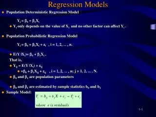
Population Deterministic Regression Model Yi = 0 + 1Xi • Yi only depends on the value of Xi and no other factor can affect Yi . • Population Probabilistic Regression Model Yi = 0 + 1Xi + i, i = 1, 2, ... , n. • E(Y |Xi)= 0 + 1Xi , That is, • Yij = E(Y |Xi) + ij • =0 + 1Xij + ij, i = 1, 2, ... , n; j = 1, 2, ... , N. • 0 and 1 are population parameters • 0 and 1 are estimated by sample statistics b0 and b1 • Sample Model: Regression Models
Assumptions Underlying Linear Regression– for Y • For each value of X, there is a group of Y values, and these Y values are normally distributed. • The means of these normal distributions of Y values all lie on the straight line of regression. • The error variances of these normal distributions are equal (Homoscedasticity). If the error variances are not constant ( called heteroscedasticity). • The Y values are statistically independent. This means that in the selection of a sample, the Y values chosen for a particular X value do not depend on the Y values for any other X values.
Sum of Squares Error Standard Error of the Estimate Standard Error of the Estimate
Sum of Squares Error Standard Error of the Estimate Proof: Standard Error of the Estimate
12-10 Coefficient of Determination • The Coefficient of Determination, r2 - the proportion of the total variation in the dependent variable Y that is explained or accounted for by the variation in the independent variable X. • The coefficient of determination is the square of the coefficient of correlation, and ranges from 0 to 1.
12-20 p.483 Confidence Interval—predict • The confidence interval for the mean value of Y for a given value of X is given by:
12-21 p.484 Prediction Interval of an individual value of Y0 • The prediction interval for an individual value of Y for a given value of X is given by:
Confidence Intervals for YX Y Confidence Intervals for E(YX) X=6.5 Figure: Confidence Intervals for Estimation
The Coefficient of Correlation, r • The Coefficient of Correlation(r) is a measure of the strength of the relationship between two variables. • It requires interval or ratio-scaled data (variables). • It can range from -1.00 to 1.00. • Values of -1.00 or 1.00 indicate perfect and strong correlation. • Values close to 0.0 indicate weak correlation. • Negative values indicate an inverse relationship and positive values indicate a direct relationship.
p.489 For sample For population (Pearson Product-Moment ) Correlation Coefficient
p. 493 Covariance
