Regression Models
Regression Models. Residuals and Diagnosing the Quality of a Model. Visualizing Regression Models. Criteria of quality. Residuals (or what we don’t explain) should be “noise” Independent variables measure different phenomena We haven’t left out something important.

Regression Models
E N D
Presentation Transcript
Regression Models Residuals and Diagnosing the Quality of a Model
Criteria of quality • Residuals (or what we don’t explain) should be “noise” • Independent variables measure different phenomena • We haven’t left out something important.
Diagnosing the Quality of a Regression Model Using the Residuals • Regression models assume that the errors of prediction are: • homoscedastic, • not autocorrelated, • normally distributed, and • not correlated with the independent variables.
Regression Models assume… • The independent variables measure different phenomena, that is the independent variables are not themselves correlated. • If they are, we have a problem of “collinearity” or “multicolinearity.”
Models • A Model: A statement of the relationship between a phenomenon to be explained and the factors, or variables, which explain it. • Steps in the Process of Quantitative Analysis: • Specification of the model • Estimation of the model • Evaluation of the model
Thus far… • We’ve discussed… • The specification of a model, • The estimation of a model and how to read and interpret the statistics we’ve produced: coefficients, t tests, F tests, R Square • Now we need to evaluate the model for problems and further elaboration.
We need to evaluate • The variation in the predicted values and the difference between the Yi and the predicted Y. That difference is called a “residual.” • We can analyze the residuals to see how good the equation is, and whether there are problems with the model that need correction or improvement.
More statistics… • Standard Error of the Estimate: The square root of the average squared error of prediction is used as a measure of the accuracy of prediction. • For the population: • For the sample:
Standard Error of the Estimate • Used to calculate a confidence interval around the predicted y. • As a rule of thumb, multiply the SEE by 2 and add and subtract from the predicted Ys to determine a measure of the variability of the prediction at a 95% confidence level. • At the mean of the independent variable: the standard error of the prediction = SEE/(square root of n).
residual is 6.2 60 55 50 predicted value is 48.8 40 Y 30 20 10 X 0 10 20 Hypothetical Example
Example from last week…. Newval = a + b1(Newsize) + b2(Families) + b3(Eastside) + b4(South) Dep Var: NEWVAL N: 467 Multiple R: 0.75 Squared multiple R: 0.56 Adjusted squared multiple R: 0.55 Standard error of estimate: 19.61 Effect Coefficient Std Error Std Coef Tolerance t P(2 Tail) CONSTANT -3.32 2.95 0.00 . -1.13 0.26 NEWSIZE 23.60 1.32 0.67 0.68 17.88 0.00 FAMILIES -5.27 2.15 -0.08 0.87 -2.46 0.01 EASTSIDE 14.06 2.53 0.20 0.78 5.56 0.00 SOUTH 6.08 2.75 0.08 0.81 2.21 0.03
To understand the principles, let’s simplify…. • We return to the bivariate case: • House value is a function of the size of the building. • Regression models assume that the errors of prediction are homoscedastic, not autocorrelated, normally distributed, and not correlated with the independent variables. • That is, the error term should be noise. • Now we ask: • 1. how accurate our prediction is, • 2. what are the characteristics of the residuals or the error term.
Model of Housing Values and Building Size Dep Var: NEWVAL N: 467 Multiple R: 0.719 Squared multiple R: 0.517 Adjusted squared multiple R: 0.516 Standard error of estimate: 20.419 Effect Coefficient Std Error Std Coef Tolerance t P(2 Tail) CONSTANT -8.667 2.012 0.000 . -4.307 0.000 NEWSIZE 25.381 1.138 0.719 1.000 22.312 0.000 Analysis of Variance Source Sum-of-Squares df Mean-Square F-ratio P Regression 207571.306 1 207571.306 497.842 0.000 Residual 193878.246 465 416.942
95% Confidence Intervals for Mean Predictions of Y (left) and Individual Predictions of Y (right)
residual is 6.2 60 55 50 predicted value is 48.8 40 Y 30 20 10 X 0 10 20 Hypothetical Example
Analysis of Residuals • ESTIMATE NEWVAL RESIDUAL • N of cases 467 467 467 • Minimum -2.647 6.400 -56.140 • Maximum 157.129 399.600 242.471 • Range 159.777 393.200 298.611 • Sum 14463.200 14463.200 0.000 • Median 25.391 24.000 -0.092 • Mean 30.970 30.970 0.000 • 95% CI Upper 32.963 33.639 1.775 • 95% CI Lower 28.977 28.301 -1.775 • Std. Error 1.014 1.358 0.903 • Standard Dev 21.917 29.351 19.522 • Variance 480.353 861.480 381.127 • C.V. 0.708 0.948 9.54775E+14 • Skewness(G1) 1.337 6.756 7.030 • SE Skewness 0.113 0.113 0.113 • Kurtosis(G2) 2.875 67.925 79.001 • SE Kurtosis 0.225 0.225 0.225

