Feedback EDF Scheduling Exploiting Dynamic Voltage Scaling
Feedback EDF Scheduling Exploiting Dynamic Voltage Scaling. Yifan Zhu and Frank Mueller Department of Computer Science Center for Embedded Systems Research North Carolina State University. Overview. Motivation Background Feedback-DVS Example Experiments Summary. Motivation.

Feedback EDF Scheduling Exploiting Dynamic Voltage Scaling
E N D
Presentation Transcript
Feedback EDF Scheduling Exploiting Dynamic Voltage Scaling Yifan Zhu and Frank Mueller Department of Computer Science Center for Embedded Systems Research North Carolina State University
Overview • Motivation • Background • Feedback-DVS • Example • Experiments • Summary
Motivation • Embedded systems w/ limited power supply • DVS for real-time system • trade-off: energy saving vs. timing requirements • lower CPU voltage/frequency deadline may miss • Task workloads change dynamically • WCET overestimates actual execution time • wide variation of execution times • Longest vs. shortest times
Motivation • Real-world examples: • graphics: 78% of WCET [Wegener,Mueller]; • defense: 87%; automotive: 74%; • benchmarks: 30-89%; image recognition: 85% [Wolf] • Prior DVS algorithms: lack adaptability to dynamic workloads. Look-ahead DVS [Pillai/ Shin]
Background • DVS: • E ~ f V² • Hard real-time systems • periodic, preemptive, independent tasks [Liu, Layland] • jobs: periodically released instances of a task • WCET: measured at full freq., w/o DVS • most practical system: U << 1 • Earliest-deadline-first (EDF) scheduling • , Ci=WCET, Pi=period • , = (0< 1) scaled by frequency
Feedback-DVS Framework • V/F selector: error c – Ca • Ca = func(error) Fig. Feedback-DVS Framework • Maximum EDF schedule • determine slack in EDF schedule • assumes: c = WCET
Voltage-Frequency Selector • : • Greedy scheme: • assign all idle time/slack to running task • Assuming all other tasks at the maximal freq. (speed) • Capitalize on early completion of current task • early completion more slack for other tasks • repeat scaling on next task
Task Splitting • T Ta + Tb • Ta at freq. ( 0 100%); Tb at freq. 100% • More aggressive: • < uniform frequency w/o splitting • Objective: • T should finish before Tb • lower energy consumption • Solve for • Ck = Ca+Cb (w/o slack) • Ck+slack = Ca/+Cb = Ca/(Ca+slack) f 100% Tb Ta t Ca/ Cb
Slack Collection • Static and dynamic slack • U<100% static slack • Idle task: fills gap between actual U and 100% U • Early completion dynamic slack • Slack passing • Preemption handling • Reserve future execution time for preempted task • Avoid over-utilizing slack by high priority tasks • Backward sweep reservation
I I I I T1 T1 T2 T2 T3 0.5+2 2 1+2 Example (w/o Feedback) T1={C=3,P=8,c=2} T2={C=3,P=10,c=2} T3={C=1,P=14,c=1} IdleT={C=1,P=4,c=0} Ca=50%WCET f 100% 75% 50% 25% t 0 5 10 15 Maximal Schedule (EDF with idle task) f 100% 75% 50% 25% We can do better! t 0 5 10 15 Actual Schedule (w/o Feedback)
Feedback Control • Scaling factor: =Ca/(Ca+slack) • Feedback control: to adjust Ca • 0<Ca<=WCET • Objective: • Ca actual exec. time (c) • But actual exec. time changes dynamically • high processing demands up to some point • receding processing demands afterwards • PID Feedback control • to improve adaptability to exec. time fluctuations
PID Feedback • Controlled variable: Ca • Set point: c • System error: = c – Ca • When Ca c: • T = Ta, no Tb, entire task at low freq./speed • PID: Proportional + Integral + Derivative • Proportional control: • Integral control: • Derivative control: c + Ca Ca PID -
100% 75% 50% 25% I I I I T1 T1 T2 T2 T3 Maximal Schedule (EDF + idle task) Ca=2,s=2 Ca=2,s=2 Ca=1,s=2 Feedback Example T1={C=3,P=8,c=2} T2={C=3,P=10,c=2} T3={C=1,P=14,c=1} IdleT={C=1,P=4,c=0} f t 0 5 10 15 f 100% 75% 50% 25% t 0 3 5 6.5 10 15 f Actual Schedule without feedback 100% 75% 50% 25% t 480 485 490 495 Actual Schedule with feedback (from the 1st hyperperiod)
Algorithm Complexity • Task admission (offline): • generate maximal schedule: O(N) • N = # jobs in hyperperiod • Scheduling point (online): • O(n), n = # tasks • Task splitting overhead: • only paid when task does not complete within Ta • hardly even happens
Experiements • Frequency/Voltage levels [Puwelse et al.]: • Parameters: 3 tasks, 10 tasks, • Vary U: utilization=0.1~ 1.0 • Feedback controller • DW=1, IW=10 • Kp=0.9, I=0.08, D=0.1 • Compare: • Our feedback-DVS vs. • Look-ahead DVS [Pillai/Shin]
Result (1) c • Task exec. time pattern 1: • event-triggered activities, often observed in interrupt-driven systems job
Result (2) c • Task exec. time pattern 2: • simulating computational demands with slowly decaying tendency job
Result (3) c • Task exec. time pattern 3: • periodic fluctuating activities with peak computational demands job
Varying Task Sets Property • 10 tasks vs. 3 tasks • Varying exec. time (baseline: pattern 1)
Related Work • Feedback control real-time scheduling [C. Lu et. al.] • DVS with feedback for multimedia systems [Z. Lu et. al.] • Look-ahead DVS [Pillai/Shin] • Exploit early completion of tasks [Aydin et. al.] • Dual-frequency DVS, stochastic approach [Gruian] • Non-preempt. Blocking, dual-speed DVS [Zhang et. al.]
Conclusion • Feedback-DVS • for hard real-time systems • more aggressive by task splitting • more adaptive with feedback control • Not sensitive to particular workload characteristics • O(n) online complexity • Up to 29% more energy savings over prior work Future Work • Feedback analytical model • Real-world architecture evaluation • Systematic PID parameter tuning
I I I I I T1 T1 T2 T2 s=3 s=6 s=6 Example (w/o Feedback) T1={C=4,P=10,c=1} T2={C=4,P=14,c=1} T3={C=1,P=17,c=1} IdleT={C=1,P=4,c=0} Ca=50%WCET f 100% 75% 50% 25% T1 T3 t 0 5 10 15 Maximal Schedule (EDF with idle task) f 100% 75% 50% 25% it will be better with feedback! t 0 5 10 15 Actual Schedule (w/o Feedback)
T1 T3 I I I I I T1 T1 T2 T2 Ca=1,s=3 Ca=1,s=3 Ca=1,s=3 Feedback Example T1={C=4,P=10,c=1}, T2={C=4,P=14,c=1}, T3={C=1,P=17,c=1}, IdleT={C=1,P=4,c=0} f 100% 75% 50% 25% t 0 5 10 15 Maximal Schedule f 100% 75% 50% 25% t 0 5 10 15 Actual Schedule without feedback f 100% 75% 50% 25% t 480 485 490 495 Actual Schedule with feedback (from the 1st hyperperiod)