Download

1 / 23
330 likes | 930 Vues
Chapter IV Compressible Duct Flow with Friction.

E N D
Chapter IVCompressible Duct Flow with Friction Chapter 3 showed the effect of area change on a compressible flow while neglecting friction and heat transfer. We could now add friction and heat transfer to the area change and consider coupled effect. Instead, as an elementary introduction, this chapter treats only the effect of friction, neglecting area change and heat transfer. The basic assumptions are : 1 – Steady one-dimensional adiabatic flow. 2 – Perfect gas with constant specific heats. 3 – Constant – area straight duct. Prof. Dr. MOHSEN OSMAN
4 – Neglecting shaft-work and potential – energy changes.5 – Wall shear stress correlated by a Darcy friction factor. In effect, we are studying a Moody-type pipe-friction problem but with large changes in kinetic energy, enthalpy, and pressure in the flow. Consider the elemental duct control volume of area A and length dx in Fig. 4.1. The area is constant, but other flow properties (P, ρ, T, h, V) may vary with x. τwπD dx V V+dV P P+dP ρ → ρ+dρ T T+dT h h+dh x x+dxFig.4.1 Elemental control volume for flow in a constant area duct with friction. Prof. Dr. MOHSEN OSMAN
Application of the three conservation laws to this control volume gives three differential equations : Continuity : (4.1a) or x – momentum : (4.1b) Energy : (4.1c) Prof. Dr. MOHSEN OSMAN
Since these three equations have five unknowns, P, ρ, T, V and τw , we need two additional relations. One is the perfect–gas law (4.2) To eliminate τw as an unknown, it is assumed that wall shear is correlated by a local Darcy factor f (4.3) Equations (4.1) and (4.2) are first-order differential equations and can be integrated, using friction – factor data, from any inlet section (1), where etc., are known, to determine - , etc., along the duct. It is practically impossible to , Prof. Dr. MOHSEN OSMAN
eliminate all but one variable to give, say, a single differential equation for P(x), but all equations can be written in terms of the Mach number M(x) and the friction factor, using the definition of Mach number. (4.4) Prove for extra class-work bonus marks ! By eliminating variables between equations (4.1) to (4.4), we obtain the working relations: (4.5a) (4.5b) Prof. Dr. MOHSEN OSMAN
Due Date : next week lecture All these except have the factor (1 - M2 ) in the denominator, so that, like the area–change formula, subsonic and supersonic flow have opposite effects. Prof. Dr. MOHSEN OSMAN
… We have added to the list above that entropy must increase along the duct for either subsonic or supersonic flow as a consequence of the second law of thermodynamics for adiabatic flow. For the same reason, stagnation pressure and density (Po , ρo ) must both decrease. The key parameter above is the Mach number whether the inlet flow is subsonic or supersonic, the Mach number always tends downstream toward M=1 because this is the path along which the entropy increases. If the pressure and density are computed from Eqs. (4.5a) and (4.5b) and the entropy from the perfect–gas relation. Prof. Dr. MOHSEN OSMAN
, the result can be plotted in Fig 4.2versus Mach number for γ = 1.4. The maximum entropy occurs at M=1, so that the second law requires that the duct–flow properties continually approach the sonic point. Fig. (4.2) Adiabatic Frictional Flow in a constant–area duct always approaches M=1 to satisfy the second law of thermodynamics. Prof. Dr. MOHSEN OSMAN
Example 4.1Air flows subsonically in an adiabatic 1-inch-diameter duct. The average friction factor is 0.024. What length of duct is necessary to accelerate the flow from M1 = 0.1 to M2 = 0.5 ? What additional length will accelerate it to M3 = 1.0 ? Assume γ = 1.4 SolutionEquation (4.8) applies, with values of computed from Eqn. (4.7) or read from Fanno- line flow Table Prof. Dr. MOHSEN OSMAN
For M3 = 1.0 Duct Length = L* @ M = 0.1i.e., the additional length to go from M = 0.5 to 1.0 is taken directly from the Table Formulae for other flow properties along the duct can be derived from Equations (4.5). Equation (4.5e) can be used to eliminate from each of the other relations, giving, for example, as a function only of M and . For convenience in tabulating the results, each expression is then integrated all the way from (P,M) to the sonic point (P*, 1.0). The integral results are: Prof. Dr. MOHSEN OSMAN
Eq. (4.5e) Substitute into equation (4.5a) Prof. Dr. MOHSEN OSMAN
Accordingly,Similarly: Prof. Dr. MOHSEN OSMAN
-- To derive working formulae, we first attack Eq. (4.5e) which relates Mach number to friction. Separate the variables and integrate, Prof. Dr. MOHSEN OSMAN
-- Prof. Dr. MOHSEN OSMAN
All these ratios are also tabulated in the same Fanno Flow Table. For finding changes between points M1 and M2 which are not sonic, products of these ratios are used. For example Example 4.2For the duct flow of Example 4.1 assume that at M1 = 0.1 we have P1 = 100 psia and T1 = 600 oR. Compute at section 2 further downstream (M2 = 0.5) (a) P2 ; (b) T2 ; (c) V2 ; (d) Po2Solution:As preliminary information we can compute V1 and Po1 from the given information: V1 =M1 C1 = M1 x49 = 0.1x49 =120 ft/s From Isentropic Table @ M=M1 =0.1 Prof. Dr. MOHSEN OSMAN
ThenNow enter Fanno Line Table, to find the following ratios Use these ratios to compute all properties downstream:Note the 77% reduction in stagnation pressure due to friction. Prof. Dr. MOHSEN OSMAN
Choking Due To FrictionThe theory here predicts that for adiabatic frictional flow in a constant area duct, no matter what the inlet Mach number M1 is, the flow downstream tends toward the sonic point. There is a certain duct length L*(M1) for which the exit Mach number will be exactly unity. But what if the actual duct length L is greater than the predict-ed “maximum” length L* ? Then the flow condition must change and there are two classifications. Subsonic Inlet If L ˃ L*(M1), the flow slows down until an inlet Mach number M2 is reached such that L = L*(M2). The exit flow is sonic and the mass flow has been reduced by frict- ional choking. Further increases in duct length will continue to decrease the inlet Mach number M and mass flux. Prof. Dr. MOHSEN OSMAN
Supersonic Inlet From Table we see that friction has a very large effect on supersonic duct flow. Even an infinite inlet Mach number will be reduced to sonic conditions in only 41 diameters for @ M = 10 @ M = ∞ Fig. (4.3) Behavior of duct flow with a nominal supersonic inlet condition M = 3.0 (a) L/D ≤ 26, flow is supersonic throughout duct; (b) L/D = 40 ˃L*/D; normal shock at M = 2.0 with subsonic flow then accelerating to sonic exit point. Prof. Dr. MOHSEN OSMAN
(c) L/D = 53, shock must now occur at M = 2.5; (d) L/D ˃ 63, flow must be entirely subsonic and choked at exit Some typical numerical values are shown in Fig. (4.3), assuming an inlet M = 3.0 and . For this condition L* = 26 diam. If L is increased beyond 26 D, the flow will not choke but a normal shock will form at just the right place for the subsequent subsonic frictional flow to become sonic exactly at the exit. Figure (4.3) shows two examples, for As length increases, the required shock moves upstream until, for Fig.(4.3), the shock is at the inlet for Further increase in L causes the shock to move upstream of the inlet into the supersonic nozzle feeding the duct. Yet the mass flux is still the same as for the very short duct, because presumably the feed nozzle still has a sonic throat. Prof. Dr. MOHSEN OSMAN
Eventually, a very long duct will cause the feed-nozzle throat to become choked, thus reducing the duct mass flux. Thus supersonic friction changes the flow pattern if L ˃L* but does not choke the flow until L is much larger than L*. Example 4.3 Air enters a 3-cm-diameter duct at and V1 = 100 m/s. The friction factor is 0.02. Compute (a) the maximum duct length for this condition, (b) the mass flux if the duct length is 15 m, and (c) the reduced mass flux if L = 30 m. Required: D = 3 cm & f = 0.02(a) Lmax for given condition (b) for L = 15 m Po =200 kPa (c) for L = 30 m To =500 K V1 = 100 m/s Prof. Dr. MOHSEN OSMAN
Solution (a) Apply energy equation between stagnation and inlet states CP To = CP T1 + ½ V12Interpolating into Fanno-Line Table across, from M=M1=0.225 we get Prof. Dr. MOHSEN OSMAN
(b) The given L=15 m is less than Lmax, and so is not choked and the mass flux follows from inlet conditions; Prof. Dr. MOHSEN OSMAN
(c) Since L = 30 m is greater than Lmax, the duct must choke back until L = Lmax, corresponding to a lower inlet M1 Interpolation in Fanno-Line Table we find that this value of 20 corresponds to M1, choked = 0.174 (23% less) From Isentropic Table : Prof. Dr. MOHSEN OSMAN