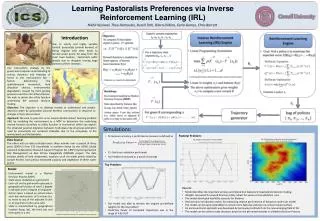
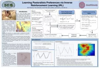
Active Learning for Reward Estimation in Inverse Reinforcement Learning

1. Active Learning for Reward Estimation in Inverse Reinforcement Learning M. Lopes (ISR)Francisco Melo (INESC-ID)L. Montesano (ISR)

2. Learning from Demonstration • Natural/intuitive • Does not require expert knowledge of the system • Does not require tuning of parameters • ... 2

3. The RL paradigm: The IRL paradigm: EXPERT WORLD Demo (Policy) Reward Agent Agent Task description (reward) Policy Inverse Reinforcement Learning 3

4. However... • IRL is an ill-defined problem: • One reward  multiple policies • One policy  multiple rewards • Complete demonstrations often impractical By actively querying the demonstrator, ... • The agent gains the ability to choose “best” situations to be demonstrated • Less extensive demonstrations are required 4

5. Outline • Motivation • Background • Active IRL • Results • Conclusions 5

6. Markov Decision Processes A Markov decision process is a tuple (X, A, P, r, γ) • Set of possible states of the world: X = {1, ..., |X|} • Set of possible actions of the agent: A = {1, ..., |A|} • State evolves according to probabilities P[Xt + 1 = y | Xt = x, At = a] = Pa(x, y) • Reward r defines the task of the agent 6

7. Example • States: 1, ..., 20, I, T, G • Actions: Up, down, left, right • Transition probabilities: Probability of moving between states • Reward: “Desirability” of each state • Goal: • Get the cheese • Avoid the trap 7

8. From Rewards to Policies • A policy defines the way the agent chooses actions: P[At = a | Xt = x] = π(x, a) • The goal of the agent is to determine the policy that maximizes the total (expected) reward: V(x) = Eπ[∑tγt rt | X0 = x] • The value for the optimal policy can be computed using DP: V *(x) = r(x) + γ maxaEa[V *(y)] Q*(x, a) = r(x) + γEa[V *(y)] 8

9. Inverse Reinforcement Learning • Inverse reinforcement learning computes r given π • In general • Many rewards yield the same policy • A reward may have many optimal policies • Example: When r(x) = 0, all policies are optimal • Given a policy π, IRL computes r by “inverting” Bellman equation 9

10. Probabilistic View of IRL • Suppose now that agent is given a demonstration: D = {(x1, a1), ..., (xn, an)} • The teacher is not perfect (sometimes makes mistakes) π’(x, a) = e n Q(x,a) • Likelihood of observed demo: L(D) = ∏iπ’(xi, ai) 10

11. Gradient-based IRL (side note...) • We compute the maximum-likelihood estimate for r given the demonstration D • We use a gradient ascent algorithm: rt + 1 = rt + r L(D) • Upon convergence, the obtained reward maximizes the likelihood of the demonstration 11

12. Active Learning in IRL • Measure uncertainty in policy estimation • Use uncertainty information to choose “best” states for demonstration So what else is new? • In IRL, samples are “propagated” to reward • Uncertainty is measured in terms of reward • Uncertainty must be propagated to policy 12

13. The Algorithm General Active IRL Algorithm Require: Initial demonstration D 1: Estimate P[π | D] using MC 2: for all xX 3: Compute H(x) 4: endfor 5: Query action for x* = argmaxxH(x) 6: Add new sample to D 13

14. The Selection Criterion • Distribution P[r | D] induces a distribution on  • Use MC to approximate P[r | D] • For each (x, a), P[r | D] induces a distribution on π(x, a): μxa(p) = P[π(x, a) = p | D] • Compute per state average entropy: H(x) = 1/|A|∑aH(μxa) Compute entropy H(μxa) a1 a2a3a4 ... aN 14

15. Results I. Maximum of a Function • Agent moves in cells in the real line [-1; 1] • Two actions available (move left, move right) • Parameterization of reward function r(x) = θ1 (x – θ2) (target: θ1 = –1, θ2 = 0.15) • Initial demonstration: actions at the borders of environment: D = {(-1, ar), (-0.9, ar), (-0.8, ar), (0.8, al), (0.9, al), (1, al)} 15

16. Results I. Maximum of a Function Iteration 5 Iteration 1 Iteration 2 16

17. Results II. Puddle World • Agent moves in (continuous) unit square • Four actions available (N, S, E, W) • Must reach goal area and avoid puddle zone • Parameterized reward: r(x) = rg exp((x – μg)2 / α) + rp exp((x – μp)2 / α) 17

18. Results II. Puddle World • Current estimates (*), MC samples (.), demonstration (o) • Each iteration allows 10 queries Iteration 1 Iteration 2 Iteration 3 18

19. Results III. General Grid World • General grid world (MM grid) • Four actions available (N, S, E, W) • Parameterized reward (goal state) • For large state-spaces, MC is approximated using gradient ascent + local sampling 19

20. Results III. General Grid World • General grid world (MM grid) • Four actions available (N, S, E, W) • General reward (real-valued vector) • For large state-spaces, MC is approximated using gradient ascent + local sampling 20

21. Conclusions • Experimental results show active sampling in IRL can help decrease number of demonstrated samples • Active sampling in IRL translates reward uncertainty into policy uncertainty • Prior knowledge (about reward parameterization) impacts usefulness of active IRL • Experimental results indicate that active is not worse than random • We’re currently studying theoretical properties of Active IRL 21

22. Thank you. 22