INTRODUCTION Bob recommendations in Green Voltage Sensors

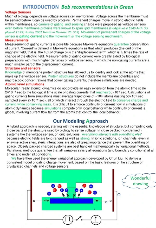
1. INTRODUCTION Bob recommendations in Green Voltage Sensors Much of biology depends on voltage across cell membranes. Voltage across the membrane must be sensed before it can be used by proteins. Permanent charges move in strong electric fields within membranes, so carriers of gating and sensing charge were proposed as voltage sensors even before membrane proteins were known to span lipid membranes (Hodgkin et al 1949 Arch. Sci. physiol 3:129;Huxley, 2002 Trends in Neurosci 25: 553). Movement of permanent charges of the voltage sensor is gating current and the movement is the voltage sensing mechanism. Measurements Measurement of gating currents is possible because Maxwell’s equations guarantee conservation of current. ‘Current’ is defined in Maxwell’s equations as that which produces (the curl of) the magnetic field, that is, the flux of charge plus the ‘displacement term’  which is ε0 times the rate of change of the electric field. Measurements of gating current were greatly aided by biological preparations with much higher densities of voltage sensors, in which the non-gating currents are a much smaller part of the displacement current. Structure and sensors Knowledge of membrane protein structure has allowed us to identify and look at the atoms that make up the voltage sensor. Protein structures do not include the membrane potentials and macroscopic concentrations that power gating currents, therefore simulations are needed. Atomic level simulations Molecular (really atomic) dynamics do not provide an easy extension from the atomic time scale 2×10-16 sec to the biological time scale of gating currents that reaches 50×10-3sec. Calculations of gating currents from simulations must average trajectories of ~1023 atoms (lasting 50×10-3sec sampled every 2×10-16 sec), all of which interact through the electric field to conserve charge and current, while conserving mass. It is difficult to enforce continuity of current flow in simulations of atomic dynamics because simulations compute only local behavior while continuity of current is global, involving current flow far from the atoms that control the local behavior. Our Modeling Approach A hybrid approach is needed, starting with the essential knowledge of structure, but computing only those parts of the structure used by biology to sense voltage. In close packed (‘condensed’) systems like the voltage sensor, or ionic solutions, ‘everything interacts with everything else’ because electric fields are long ranged as well as strong. In ionic solutions, ion channels, even in enzyme active sites, steric interactions are also of great importance that prevent the overfilling of space. Closely packed charged systems are best handled mathematically by variational methods. Variational methods guarantee that all variables satisfy all equations (and boundary conditions) at all times and under all conditions. We have then used the energy variational approach developed by Chun Liu, to derive a consistent model of gating charge movement, based on the basic features of the structure of crystallized channels and voltage sensors. Wonderful drawing

2. Mathematical Description • The axisymmetric geometric configuration is shown in Fig. 1 with being the antechambers and being the channel. Na and Cl only reside at antechambers and can not enter channel, while 4 arginines (marked 1-4) can reside at both antechambers and channel but can not further exit to the reservoirs outside. The reduced 1D dimensionless PNP-steric equations are expressed as below. The first one is Poisson equation: (1) with and A(z) being the cross-sectional area. To be specific, Valance (charge ) of ions depends on pKa of channel environment, and will be a free parameter to input. The second equation is the transport equation based on conservation law: (2) with the content of Ji based on Nernst-Planck equation: (3) and for 4 arginines ci, i=1, 2, 3 and 4, based on Fig. 2, (4) (5) (6) (7) where Di, i=Na, Cl, 1, 2, 3, and 4 are diffusion coefficients, and g is the parameter characterizing steric effect. Larger g implies larger steric effect, but g can not be arbitrarily large due to the limitation of stability. Vi, i=1, 2, 3 and 4 being the trap potential for ci

3. representing a spring connecting ci to S4 as shown in Fig. 2. Specifically, (8) where K is the spring constant, zi is the anchoring position of spring for cion S4, is the z-direction displacement of S4 by treating S4 as a rigid body. follows the motion of equation of S4 based on spring-mass system: (9) where mS4, bS4 and KS4 are mass, damping coefficient and restraining spring constant for S4. is the center of mass for ci , which is calculated by , i=1, 2, 3, 4. (10) Assuming (9) is quasi-steady, (9) can then be simplified as (11) The additional potential V in (4-7) is caused by the hydrophobic environment of channel. It can be seen as the solvation energy barrier. If we use Born model to estimate the solvation energy, , (12) where and are dielectric constants for antechamber and channel, respectively. Usually we treat , and then (here we set ). The apparent radius of the guanidinium ion, which is the ionic part of the arginine, is 0.21 nm. With zarg=1, we can therefore obtain to be close to . will actually affect only the value of transition voltage (the steep-slope regime of voltage in saturation map). So we don't have to be very serious about if is exactly correct or not. Here, we set (13) with Vmax being the free parameter to input. Note that tanh function is employed to smooth the top-hat-shape barrier profile, which is not good for differentiation. Boundary and interface conditions for electric potential are . (14) Boundary and interface conditions for arginine are (15) Boundary conditions for Na and Cl are (16)

4. Initial conditions are (17) Input parameters: LR=1, L=1, ra=1, rR=1.5, zarg=1, DNa=DCl=1, Di=1, i=1,2,3,4, Q=1/20, g=0.5, Vmax=5, z1=LR+0.5L-0.3=1.7, z2=LR+0.5L-0.1=1.9, z3=LR+0.5L+0.1=2.1, z4=LR+0.5L+0.3=2.3, K=10, KS4=80. Considering the hydrophobic environment for arginine inside the channel, we set Important parameter to be varied for investigation is . Note that is dimensionless. Multiply by 26 mV to change to dimensional units. Outputs: gating current I at z=0, LR+L/2; , are volume fraction of arginine in zone 1, 2 and 3, respectively. and time course of gating charge (time integral of gating current at z=LR+L/2) are also outputs and compared.