Download
1 / 53
530 likes | 645 Vues
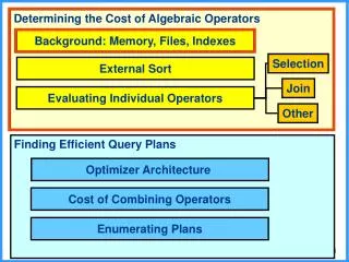
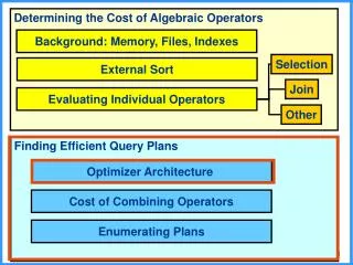
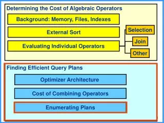
Determining the Cost of Algebraic Operators. Background: Memory, Files, Indexes. Selection. External Sort. Join. Evaluating Individual Operators. Other. Finding Efficient Query Plans. Optimizer Architecture. Cost of Combining Operators. Enumerating Plans. Relational Query Optimization.

E N D
Determining the Cost of Algebraic Operators Background: Memory, Files, Indexes Selection External Sort Join Evaluating Individual Operators Other Finding Efficient Query Plans Optimizer Architecture Cost of Combining Operators Enumerating Plans
Relational Query Optimization Enumeration of Alternative Plans
Enumeration • Up until now, we have seen examples of query plans and have estimated their costs • Now, we discuss how all plans of interest can be systematically enumerated • Discussion divided into 3 parts: • single relation queries (no join) • two relation queries (one join) • multiple relation queries (more than one join)
Single Relation Query SELECT S.rating, S.sname FROM Sailors S WHERE S.rating>5 and S.age=20 ORDER BY S.rating • When the query uses only one relation, the most important decision is how to access that relation: • full table scan • via a matching index, when available Which Choice will be Cheapest?
Single Relation Query SELECT S.rating, S.sname FROM Sailors S WHERE S.rating>5 and S.age=20 • Suppose, no indexes are available what is the cost of evaluating the query? • Note: between unary operators pipeline is always done. • 500 to read sailors • Rest is pipe lined • Note: distinct will add the efficiency of a sort
Using an Index SELECT S.rating, S.sname FROM Sailors S WHERE S.rating>5 and S.age=20 • If we do have indexes, we may be able to use them to speed up the execution • We have many choices of access paths if there are several conditions, with several matching indexes
Plans Utilizing an Index • Single-index access plans: • May be several indexes that match the selection conditions. • Optimizer chooses most selective index, reads tuples via index and performs on-the-fly selection for additional conditions • Multiple-index access plans: • Use several indexes to find rowids. Then, intersect sets of rowids and sort result. Retrieve tuples with corresponding rowids and apply remaining selections Not Considered in this Course
Plans Utilizing an Index (cont.) • Sorted-index access plans: • If list of attributes that we must sort by is prefix of a BTree key, we can retrieve the tuples in order via a BTree, and then apply additional selections. • Index-only access plans: • If all attributes mentioned in the query are in a search key for some index, can use the index alone to answer the query (without accessing the actual table!)
Example SELECT S.rating, S.sname FROM Sailors S WHERE S.rating>5 and S.age=20 ORDER BY S.rating • Ratings are between 1 and 10 • Ages are between 18 and 67 (including) • The field rating has size 10 (bytes) • The field sname has size 15 (bytes) • Buffer size is 10
Example: Single-Index Access SELECT S.rating, S.sname FROM Sailors S WHERE S.rating>5 and S.age=20 ORDER BY S.rating • Given: a clustered hash index on age, with access time 2 I/Os • What is the cost of a single-index access plan? • Remember to count the time for sorting! recoils
Example: Single-Index Access SELECT S.rating, S.sname FROM Sailors S WHERE S.rating>5 and S.age=20 ORDER BY S.rating • What is the cost of a single-index access plan? • Select s.age=20: 12 • Go over the index = 2 • Load the lines = 500/50 (1 out of 50 age values) = 10 • Select s.rating • Size after second choose = 10/2 = 5 • Size after projection = 5/3 = 3 (rating and sname are ½ of the block)
Example: Sorted-Index Access SELECT S.rating, S.sname FROM Sailors S WHERE S.rating>5 and S.age=20 ORDER BY S.rating • Given: an unclusteredBtree index on rating, with access time 3 I/Os • What is the cost of a sorted-index (single-index) access plan? Do we have to sort?
Example: Sorted-Index Access SELECT S.rating, S.sname FROM Sailors S WHERE S.rating>5 and S.age=20 ORDER BY S.rating • What is the cost of a sorted-index (single-index) access plan? Do we have to sort? • 3 + 500*80/2 = 20003
Example: Index-Only Access SELECT MAX(S.rating) FROM Sailors S • Given: an unclusteredBtree index on rating, with access time 3 I/Os • What is the time to evaluate this query? • 3
Single Join Queries • At this point, you should already be able to enumerate all query plans for single join queries (which may contain projection/selection) • Consider each join method • For block nested loops and index nested loops consider both options for inner/outer relations • Push selections/projections, when possible and cheaper • Pipeline results when possible • Access relations in cheapest ways Example
Single Join, Single Selection: Enumerating Plans • Assume that there is • An index on R.bid • An index on S.sid • What are all query plans that must be considered, given no additional constraints on the optimizer? SELECT * FROM Sailors S, Reserves R WHERE S.sid = R.sid and R.bid = 100
bid=100 On-the-fly BNL sid=sid Sailors Reserves (1) SELECT * FROM Sailors S, Reserves R WHERE S.sid = R.sid and R.bid = 100 Available: Index on R.bid Index on S.sid Block Nested Loops Join, Reserves as Outer BNL BNL BNL BNL sid=sid sid=sid sid=sid sid=sid (2) File scan. Write to T1 File scan. on-the-fly Index Write to T1 Index On-the-fly bid=100 bid=100 bid=100 bid=100 Sailors Sailors Sailors Sailors (4) Reserves Reserves Reserves Reserves (5) (3)
bid=100 On-the-fly BNL sid=sid Sailors Reserves (1) SELECT * FROM Sailors S, Reserves R WHERE S.sid = R.sid and R.bid = 100 Available: Index on R.bid Index on S.sid Block Nested Loops Join, Reserves as Outer More expensive than (4) BNL BNL BNL BNL sid=sid sid=sid sid=sid sid=sid (2) Index Write to T1 Index On-the-fly File scan. Write to T1 File scan. on-the-fly bid=100 bid=100 bid=100 bid=100 Sailors Sailors Sailors Sailors (4) Reserves Reserves Reserves Reserves More expensive than (4) (5) (3) More expensive than (5)
BNL, Selection on Outer • Always push selection on outer relation of BNL • Determining whether (4) or (5) is cheaper is simply checking whether it is more efficient to evaluate the selection using a file scan or using an index • Reduction to single relation query problem!
bid=100 On-the-fly BNL sid=sid Sailors Reserves (1) SELECT * FROM Sailors S, Reserves R WHERE S.sid = R.sid and R.bid = 100 Available: Index on R.bid Index on S.sid Block Nested Loops Join, Sailors as Outer (2) (4) BNL sid=sid BNL sid=sid File scan. Write to T1 bid=100 Sailors File scan. On-the-fly bid=100 Sailors Reserves Reserves (5) (3) BNL BNL sid=sid sid=sid Index. Write to T1 bid=100 Index On-the-fly bid=100 Sailors Sailors Reserves Reserves
bid=100 On-the-fly BNL sid=sid Sailors Reserves (1) SELECT * FROM Sailors S, Reserves R WHERE S.sid = R.sid and R.bid = 100 Available: Index on R.bid Index on S.sid Block Nested Loops Join, Sailors as Outer (2) (4) BNL sid=sid BNL sid=sid File scan. Write to T1 bid=100 Sailors File scan. On-the-fly bid=100 Pipelining not possible on Inner relation of BNL Sailors Reserves Reserves (5) (3) BNL BNL sid=sid sid=sid Index. Write to T1 bid=100 Index On-the-fly bid=100 Pipelining not possible on Inner relation of BNL Sailors Sailors Reserves Reserves
BNL, Selection on Inner • Pushing selection on inner may or may not improve the runtime • Depends on the time to write the result of the selection and • The degree to which the selection makes the inner relation smaller • Determining whether (2) or (3) is cheaper is simply checking whether it is more efficient to evaluate the selection using a file scan or using an index • Reduction to single relation query problem!
bid=100 bid=100 On-the-fly On-the-fly BNL BNL sid=sid sid=sid Sailors Reserves Sailors Reserves (1) (1) Block Nested Loops: Note • We do not have to evaluate the cost of both of these: • Sufficient to consider the plan with a smaller relation on the left
bid=100 On-the-fly INL sid=sid Sailors Reserves (1) SELECT * FROM Sailors S, Reserves R WHERE S.sid = R.sid and R.bid = 100 Available: Index on R.bid Index on S.sid Index Nested Loops Join, Reserves as Outer INL INL INL INL sid=sid sid=sid sid=sid sid=sid (2) File scan. Write to T1 File scan. on-the-fly Index Write to T1 Index On-the-fly bid=100 bid=100 bid=100 bid=100 Sailors Sailors Sailors Sailors (4) Reserves Reserves Reserves Reserves (5) (3)
bid=100 On-the-fly INL sid=sid Sailors Reserves (1) SELECT * FROM Sailors S, Reserves R WHERE S.sid = R.sid and R.bid = 100 Available: Index on R.bid Index on S.sid Index Nested Loops Join, Reserves as Outer More expensive than (4) INL INL INL INL sid=sid sid=sid sid=sid sid=sid (2) Index Write to T1 Index On-the-fly File scan. Write to T1 File scan. on-the-fly bid=100 bid=100 bid=100 bid=100 Sailors Sailors Sailors Sailors (4) Reserves Reserves Reserves Reserves More expensive than (4) (5) (3) More expensive than (5)
INL, Selection on Outer • Always push selection on outer relation of INL • Determining whether (4) or (5) is cheaper is simply checking whether it is more efficient to evaluate the selection using a file scan or using an index • Reduction to single relation query problem!
bid=100 On-the-fly INL sid=sid Sailors Reserves (1) SELECT * FROM Sailors S, Reserves R WHERE S.sid = R.sid and R.bid = 100 Available: Index on R.bid Index on S.sid Index Nested Loops Join, Sailors as Outer (2) (4) INL sid=sid INL sid=sid File scan. Write to T1 bid=100 Sailors File scan. On-the-fly bid=100 Sailors Reserves Reserves (5) (3) INL INL sid=sid sid=sid Index. Write to T1 bid=100 Index On-the-fly bid=100 Sailors Sailors Reserves Reserves
bid=100 On-the-fly INL sid=sid Sailors Reserves (1) SELECT * FROM Sailors S, Reserves R WHERE S.sid = R.sid and R.bid = 100 Available: Index on R.bid Index on S.sid Index Nested Loops Join, Sailors as Outer There is no index on Reserves.sid, so Reserves CANNOT be the inner relation in INL. If there was an index on Reserves.sid, only (1) would be feasible, since selections CANNOT be pushed to the inner relation of INL (2) (4) INL sid=sid INL sid=sid File scan. Write to T1 bid=100 Sailors File scan. On-the-fly bid=100 Sailors Reserves Reserves (5) (3) INL INL sid=sid sid=sid Index. Write to T1 bid=100 Index On-the-fly bid=100 Sailors Sailors Reserves Reserves
INL, Selection on Inner • Pushing selection on inner is not possible in INL • INL can only be applied when there is an index on the join attribute of the inner relation
bid=100 On-the-fly SMJ sid=sid Sailors Reserves (1) SELECT * FROM Sailors S, Reserves R WHERE S.sid = R.sid and R.bid = 100 Available: Index on R.bid Index on S.sid Sort Merge Join SMJ SMJ SMJ SMJ sid=sid sid=sid sid=sid sid=sid (2) File scan. Write to T1 File scan. on-the-fly Index Write to T1 Index On-the-fly bid=100 bid=100 bid=100 bid=100 Sailors Sailors Sailors Sailors (4) Reserves Reserves Reserves Reserves (5) (3)
bid=100 On-the-fly SMJ sid=sid Sailors Reserves (1) SELECT * FROM Sailors S, Reserves R WHERE S.sid = R.sid and R.bid = 100 Available: Index on R.bid Index on S.sid Sort Merge Join SMJ SMJ SMJ SMJ sid=sid sid=sid sid=sid sid=sid (2) Index On-the-fly File scan. on-the-fly File scan. Write to T1 Index Write to T1 bid=100 bid=100 bid=100 bid=100 Sailors Sailors Sailors Sailors (4) Reserves Reserves Reserves Reserves Pipelining not possible on relations of SMJ (5) (3) Pipelining not possible on relations of SMJ
Sort Merge Join • Pushing selection on may or may not improve the runtime • Depends on the time to write the result of the selection and • The degree to which the selection makes the inner relation smaller • Determining whether (2) or (3) is cheaper is simply checking whether it is more efficient to evaluate the selection using a file scan or using an index
Some Notes • Projection is dealt with in the exact same manner as selection • If there are more indexes, then some additional options may become available • E.g., index on R.sid, then Reserves as inner in INL • If there are less indexes, then some options may become available • E.g., no index on S.sid, then INL, not possible • E.g., no index on R.bid, then selection can only be performed using file scan
Some More Notes • If there is a selection on both inner and outer relations, then follow rules introduced here for both relations • We now review with another example…
Course(cid,name,points,room,lid) Lecturer(lid,name,level) SELECT * FROM Course C, Lecturer L WHERE L.lid = C.lid and C.points>3 and C.room=7 • There are 20,000 courses. 100 rows fit in a page • There are 5,000 lecturers. 200 rows fit in a page • The buffer is of size 22 • The number of points for a course is between 2 and 5 • There are 100 rooms • There is a clustered Btree on L.lid, with access time 3 • There is an unclustered Hash on C.room, with access time 2 • There is a clustered Btree on C.points, with access time 3 • What is the cheapest plan, if only BNL and INL can be used?
Course(cid,name,points,room,lid) Lecturer(lid,name,level) SELECT * FROM Course C, Lecturer L WHERE L.lid = C.lid and C.points>3 and C.room=7 • What is the cheapest plan, if only BNL and INL can be used? • Size of Course: 20000/100 = 200 blocks • Size of Lectures: 5000/200 = 25 blocks • Access Course: • File scan: 200 • Hash (room): 2 + 200*100(n lines)/100(room options) = 202 • Btree on Points: 3 + 200(total blocks)/2(half of the course have more then 3 points) = 103 (IO Reads) • Access Lectures: • File scan: 25 • (Btree: not of a value we need ) • Files after selection = 25 • Size of Course after selection: • 200(total)/2(n points selection)/100(room selection) = 1
Course(cid,name,points,room,lid) Lecturer(lid,name,level) SELECT * FROM Course C, Lecturer L WHERE L.lid = C.lid and C.points>3 and C.room=7 • Plans • BNL course on outer • Select course = 103 • Join: Br + Bs*Br / 2B = 25*[1/20] = 25 • Total 128 • INL course on outer • Select 103 • Join: 1*100 *(3(Btree) + 1(lec to each course)) = 400 • Total: 503
Course(cid,name,points,room,lid) Lecturer(lid,name,level) SELECT * FROM Course C, Lecturer L WHERE L.lid = C.lid and C.points>3 and C.room=7 • Plans • BNL Lecture on outer • We differ to 2 different ways – first with the selection before the join and second after • Select before the join • Select after the join • The select is on the fly • BR + BS ([Br]/(B-2)) • 25 + 200([25/(22-2)])=425 • Select before the join • Select with index on course: 103 • Writing to temp file = 1 • BR + BS ([Br]/(B-2)) • Total: 103 + 25+(200/200)*(25/(22-2)) = 103 + 27 = 131
Multiple-Relation Queries • When there are several relations in a query, planning becomes more complex. Some issues: • how should each relation be accessed? • in which order should relations be joined? • what join algorithms should be used? • Most optimizers only consider left-deep plans. (Why?) We will only discuss enumerating of left-deep plans
Enumeration of Left-Deep Plans • System R style optimizers (which we discuss here) consider left-deep plans with selection and projections considered as early as possible. It also avoids cartesian products, when possible • selections sometimes will not be pushed, if they cannot be performed on-the-fly • Enumeration is a multi-pass algorithm SELECT attribute list FROM relation list WHERE term1and … and termn
Enumeration of Left-Deep Plans: Pass 1 • Enumerate all single-relation plans, for each relation in the FROM clause • May be several ways to access each relation R • When finding a plan, consider: which conditions in the WHERE clause are selections on R, and which attributes can be projected out early • Find and retain cheapest plan. • If plans return tuples in some sorted order, also return a cheapest plan for each sorted order that can be produced.
Enumeration of Left-Deep Plans: Pass 2 • Enumerate all 2-relation plans, by: • consider each single relation plan from Pass 1 as an outer relation R • consider each join algorithm available in the database • consider each relation S that has a join condition with R. Determine best access method for S, considering the type of join of interest. (mostly enumerated in previous pass) • Find and retainall cheapest 2-relationplans. • If plans return tuples in some sorted order, also return a cheapest plan for each sorted order.
Enumeration of Left-Deep Plans: Pass 3 • Generate all 3-relation plans. • Continue as before, but consider all results of the previous stage as possible outer relations. Continue as needed, for additional passes until complete plans are generated
Example SELECT * FROM Sailors S, Reserves R, Boats B WHERE S.sid = R.sid and R.bid = B.bid and R.bid = 100 • Our single relation access plans will find best ways to access Sailors, Reserves, Boats • Our 2-relation plans will consider best plans for joining • Sailors and Reserves • Reserves and Boats • Our final plans will find best ways to join with remaining relation
bid=100 On-the-fly SMJ sid=sid Sailors Reserves (b) For example • Suppose that the following 2 relation plans were retained (i.e., were the cheapest) (a) BNL sid=sid File scan. on-the-fly bid=100 Boats Reserves
bid=100 On-the-fly SMJ sid=sid Sailors Reserves (b) Then … • We find the best plan to join Sailors with: • And the best plan to join Boats with: • And keep the best of these (a) BNL sid=sid File scan. on-the-fly bid=100 Boats Reserves
Two Tricky Issues • There are 2 tricky issues that you have to be careful about when computing the cost of a multi-relation join: • Estimating the size of the output of a join • When pipelining results from the first join into the second, the buffer must be allocated for 3 relations (not 2) • We will demonstrate both of these issues with an example…