Download

1 / 61
610 likes | 659 Vues
Explore the evolutionary relationships among gene sequences and organisms through sequence analysis in bioinformatics. Understand the importance of aligning sequences and constructing phylogenetic trees in understanding the Tree of Life.

E N D
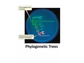
Phylogenetic Trees using Sequence Analysis to investigate the Tree of Life Stephen Sontum Middlbury College sontum@middlebury.edu Chapter 5: Alignments and Phylogenetic Trees Introduction to Bioinformatics Chapter 3: Evolution and Genomic Change Introduction to Genomics
What we hope to learnPhylogenetic Trees • Evaluation of the sequence alignment- Gap penalties- Local vs Global Alignment- E values • Clustering Data- Evolution- Phylogenetic Trees • Web Pages Core
A Parts List Approach to Baby Maintenance Clearly this is a much larger informatics problem but we can begin in the same way by finding and organizing the parts. Evolution is one of the best ways to organize the parts. TGAATCCCAGTTCAGCTCTTCAGCCTTTCGTGGATAAGAGAAGGCTGAAAGCGGGTCACGTTTTGGACTAAGCGACGCCC TTGCCAGGCATCCAGCTTAGTGGCTGTTGGTTTATTTGTAGAGTCCCCTTAACTCTCTCTCCCCCACATCGCCCATCTCC ACCGACGCCTCTCTCTCTCGTGTTATTTCTCCCCATTCTCGCTTCATTTCCCATCCATTTTCGAGTTCTGCAATATCCTC ACTAACTAGTATAGCCATGGTACGCCTCACTCGATCATCATCGTTGTTCGTGCGCTCAAACGCATCCGCTGTGCGGGGCA GATCTACTGGTGTCCTCCTGCGTAGATGAGCTGACGACTTCACTTCCAGGCCGACTCTCTGACCGAAGAGCAAGTTTCCG AGTACAAGGAGGCCTTCTCCCTATTTGTAAGTGCCATTGGTTACTGTTATATCAAAATCGAATTTGTATTGAGAGTATAC TAATACATTCCGCACTAAACAGGACAAGGATGGCGATGGTTAGTGCATCTGTCCCCCCAGGCTTGATCGCATTCGCCCAG CATGTCTGCTGTAGCTCTATATAACCGTTTCTGACAAACGGCGACAGGCCAGATTACCACTAAGGAGCTTGGCACTGTCA TGCGCTCGCTCGGTCAGAATCCTTCAGAGTCTGAGCTTCAGGACATGATCAACGAAGTTGACGCCGACAACAATGGCACC ATTGACTTTCCAGGTACGCGAACTCCCCAATCTACTTCGCACCAGCCTAGAAATGTACTAATGCTAAACAGAGTTCCTTA CCATGATGGCCAGAAAGATGAAGGACACCGATTCCGAGGAGGAAATTCGGGAGGCGTTCAAGGTCTTCGACCGTGACAAC AATGGTTTCATCTCCGCTGCTGAGCTGCGTCACGTCATGACCTCGATCGGTGAGAAGCTCACCGATGACGAAGTCGACGA
Evolution • The theory of evolution is the foundation upon which all of modern biology is built. • From anatomy to behavior to genomics, the scientific method requires an appreciation of changes in organisms over time. • It is impossible to evaluate relationships among gene sequences without taking into consideration the way these sequences have been modified over time
Relationships Similarity searches and multiple alignments of sequences naturally lead to the question: • “How are these sequences related?” • “How are the organisms from which these sequences come related?”
Taxonomy • The study of the relationships between groups of organisms is called taxonomy, an ancient and venerable branch of classical biology. • Taxonomy is the art of classifying things into groups — a quintessential human behavior — established as a mainstream scientific field by Carolus Linnaeus (1707-1778).
DNA is a good tool for taxonomy DNA sequences have many advantages over classical types of taxonomic characters: • Character states can be scored unambiguously • Large numbers of characters can be scored for each individual • Information on both the extent and the nature of divergence between sequences is available (nucleotide substitutions, insertion/deletions, or genome rearrangements)
What Can Happen to a Gene During Evolution: • A gene may pass to descendants, accumulating favorable or unfavorable mutations or drift neutrally. • A gene may be lost. • A gene my be duplicated, followed by divergence or loss of one of a pair. • A gene may undergo horizontal transfer to an organism or another species. • A gene may undergo complex patters of fusion, fission, or rearrangement
What Can Happen to a Gene During Evolution: Figure 2.12 Thioredoxins are proteins that catalyze disulfide-exchange reactions, contributing to the speed and accuracy of the protein-folding process. Note the gaps (deletions or insertions).
Sequences Reflect Relationships • After working with sequences for a while, one develops an intuitive understanding that for a given gene, closely related organisms have similar sequences and more distantly related organisms have more dissimilar sequences. • Given a set of gene sequences, it should be possible to reconstruct the evolutionary relationships among genes and among organisms. • These differences or evolutionary distances between genes can be quantified by scoring their Pair-wise alignment.
Parameters for Scoring Alignment • Scoring Systems: • Each symbol pairing is assigned a numerical value, based on a symbol comparison table. • Gap Penalties: • Opening: The cost to introduce a gap • Extension: The cost to elongate a gap Core
actaccagttcatttgatacttctcaaa taccattaccgtgttaactgaaaggacttaaagact DNA Scoring Systems -very simple Sequence 1 Sequence 2 A G C T A1 0 0 0 G 0 1 0 0 C 0 0 1 0 T 0 0 0 1 Match: 1 Mismatch: 0 Score = 5
Scoring Insertions and Deletions A T G T A A T G C A T A T G T G G A A T G A A T G T - - A A T G C A T A T G T G G A A T G A insertion / deletion The creation of a gap is penalized with a negative score value.
Why Gap Penalties? Gaps not permitted Score: 0 1 GTGATAGACACAGACCGGTGGCATTGTGG 29 ||| | | ||| | || || | 1 GTGTCGGGAAGAGATAACTCCGATGGTTG 29 Match = 14Mismatch = -14 Gaps allowed but not penalized Score: 20 1 GTG.ATAG.ACACAGA..CCGGT..GGCATTGTGG 29 ||| || | | | ||| || | | || || | 1 GTGTAT.GGA.AGAGATACC..TCCG..ATGGTTG 29
Why Gap Penalties? • The optimal alignment of two similar sequences is usually that which • maximizes the number of matches and • minimizes the number of gaps. • There is a tradeoff between these two • - adding gaps reduces mismatches • Permitting the insertion of arbitrarily many gaps can lead to high scoring alignments of non-homologous sequences while large gap penalties reduce homology. • “Affine” gap penalties balance these consideration by allowing extensions of a gap
actaccagttcatttgatacttctcaaa tacca-ttaccgtgttaactg--aaaggacttaaagact actaccagttcatttgatacttctcaaa tacca-ttaccgtgttaactgaaaggacttaaagact DNA Scoring Systems - Affine Sequence 1 Sequence 2 a) Match: 2 b) Mismatch: 2 c) Gap initiation: 5 d) Gap extension: 2 R = a I - b X - c O – d G R = 2*15 – 2*8 – 5*2 – 2*3 R = -2 R = 2*13 – 2*12 – 5*1 – 2*1 R = -5 For global alignment we count end gaps but for local we do not.
Global vs. Local Alignments • Global alignment algorithms start at the beginning of two sequences and add gaps to each until the end of one is reached. • Local alignment algorithms finds the region (or regions) of highest similarity between two sequences and build the alignment outward from there.
Global vs. Local Alignment TTGACACCCTCCCAATTGTA ACCCCAGGCTTTACACAT NW (Needleman & Wunsch)creates an end-to-end alignment. TTGACACCCTCCCAATTGTA--- |||| || | -----ACCCCAGGCTTTACACAT SW (Smith-Watterman)creates an local alignment. ---------TTGACACCCTCCCAATTGTA || |||| ACCCCAGGCTTTACACAT-----------
Local Alignment Two sequences sharing several regions of local similarity: 1 AGGATTGGAATGCTCAGAAGCAGCTAAAGCGTGTATGCAGGATTGGAATTAAAGAGGAGGTAGACCG.... 67 |||||||||||||| | | | |||| || | | | || 1 AGGATTGGAATGCTAGGCTTGATTGCCTACCTGTAGCCACATCAGAAGCACTAAAGCGTCAGCGAGACCG 70 Local similarities may occur in sequences with different structure or function that share common substructure/subfunction. MOTIFS… Local Alignments are better representations of Evolution.
Global Alignment (Needleman -Wunsch) • Global algorithms are often not effective for highly diverged sequences - do not reflect the biological reality that two sequences may only share limited regions of conserved sequence. • Sometimes two sequences may be derived from ancient recombination events where only a single functional domain is shared. • Global methods are most useful when you want to force two sequences to align over their entire length
D-P modifications for Local Alignment (Smith-Waterman) Smith TF, Waterman MS “Identification of Common Molecular Subsequences” J. Mol Biol. 147: 195-197 (1981) • The scoring system uses negative scores for mismatches. • The minimum score for [i,j] is zero. • The best score is sought anywhere in matrix (not just last column or row) These three changes cause the algorithm to seek high scoring subsequences, which are not penalized for their global effects (mod 2),which don’t include areas of poor match (mod 1)and which can occur anywhere (mod 3).
Comparison of Methods • SW, FASTA and BLAST: local alignments • NW: global alignments • Speed: BLAST > FASTA > NW >> SW • Sensitivity: SW > FastA >= BLAST- FastA gives better separation between homologs and random hits Core
BLAST is Approximate • BLAST makes similarity searches very quickly because it takes shortcuts. • looks for short, nearly identical “words” (11 bases or 2-3 amino acids) • It also makes errors • misses some important similarities • makes many incorrect matches • easily fooled by repeats or skewed composition
Blast produces HSPs • The results of the word matching and attempts to extend the alignment using SW are segments • called HSPs (High-scoring Segment Pairs) • HSPssignificance can be statistically evaluated
Blast Matches are Ranked by E BLASTN results on BE588357 Bos taurus cDNA >dbj|AK170263.1| Gene info linked to AK170263.1 Mus musculus Score = 48.2 bits(52),Expect= 0.037 Identities = 32/35 (92%), Gaps = 2/35 (5%) Strand=Plus/Plus Query 48 GCAGCCATGGCCAGCAAGGGCTTGCAGGACCTGAA 82 ||||||| ||||||||||| |||||||||||||| Sbjct 396 GCAGCCA--GCCAGCAAGGGTTTGCAGGACCTGAA 428 Alignment: only a small section of Bos taurus aligned Search Summary Match/Missmatch scores = 2, -3 Gap costs = 5,2 Effective length of query = 334 Effective length of database = 35244975650 Karlin-Altschul statistics Lamba = 0.633731 gapped 0.625Kapa = 0.408146 gapped 0.78 Bit Score = 48.2 Raw Score = 52 E-value = 0.037 Identities = 92%
Bit Score and Raw Score >dbj|AK170263.1| Gene info linked to AK170263.1 Mus musculus Score = 48.2 bits(52),Expect= 0.037 Identities = 32/35 (92%), Gaps = 2/35 (5%) Strand=Plus/Plus Query 48 GCAGCCATGGCCAGCAAGGGCTTGCAGGACCTGAA 82 ||||||| ||||||||||| |||||||||||||| Sbjct 396 GCAGCCA--GCCAGCAAGGGTTTGCAGGACCTGAA 428 • Raw score (alignment similarity) RR = a I + b X – c O – d G (for Nucleic Acids)I identities, X mismatches, O #gaps, G # ”-”Rij = ln(Pij/Pi Pj)/λ (scoring matrix for proteins) • Bit score (normalized Similarity) Sif we were to represent the alignment information as a binary number it would be 48 bits long 111111100111111111011111111111111001101010011100
What is an E-Value • Statistics of High Scoring Segment Pairs HSPs • E-value number of random alignments with bit scores greater than S E = K n m e−λR = n m 2−S S = (λ R – ln K)/ln 2 http://www.ncbi.nlm.nih.gov/BLAST/tutorial/Altschul-1.html The Statistics of Sequence Similarity Scores • K and λ are constants like the average and standard deviation that normalize the E and S values and depend on how the alignments were scored
What is an E-Value λ R – ln K E = n m 2−S S = • E the number of random alignments with bitscores > S • Larger S is less likely to occur from chance, corresponding to smaller E values • Because a particular bit score is more easily obtained by chance with a longer query m, longer queries correspond to larger E value • Because a larger database n makes a particular bit score more easily obtained by chance, larger n results in a larger E value. ln 2
N(s,m,x) = e What is a P-Value Errorbound - (x – m)2 2 s2 Normal Distribution 1 s√2p ± Z s P(Random Z score ≥ 2) = 2.5 % Probability is represented by area under the Distribution Normalizedscore
What in a P-Value -E P(Random score ≥ S) = 1 – e • Z-score of S Z=0 no better than average Z > 5 significant match • P–value P < 10-100 exact match P < 10-10 closely related P < 10-1 distant relatives P > 10-1 insignificant • E-value E < 0.02 probably homologous E < 1 homology unproven E > 1 random match Counting experiments follow a non symmetric Poisson Distribution
Interpretation of E-values • very low E() values (e-100) are homologs or identical genes • moderate E() < 0.02 values are related genes • long list of gradually declining of E() values indicates a large gene family • long regions of moderate similarity are more significant than short regions of high identity
Tips for DB searches • Run Blast first, then depending on your results run a finer tool (FastA,SW) • Where possible use protein sequence. • E() < 0.05 is statistically significant, and usually biologically interesting. • Matches of >50% identity in a 20-40 amino acid region occur frequently by chance.
Tips for DB searches If the query has repeated segments, remove them and repeat the search. Split large query sequence( if >1000 for DNA, >200 for protein). Pay attention to abnormal composition of the query sequence, it usually causes biased scoring.
Phylogenetic Trees using Sequence Analysis to Investigate the Tree of LifeFirst lecture Ended Here • Clustering Data- Evolution- Phylogenetic Trees • Web Pages
Biodiversity and Conservation Check out the Tree of Life project for an introduction to phylogenetics and its relationship to biodiversity. http://phylogeny.arizona.edu/tree/phylogeny.html Measurements of DNA sequence differences are now being used to implement plans for the conservation of genetic resources.
Phylogenetics • Evolutionary theory states that groups of similar organisms are descended from a common ancestor. • Cladistic approach is a method of taxonomic classification (cladogram) based on their evolutionary history. • Phenetic approach construct trees (phenograms) by considering the current distance between the states of characters without regard to the evolutionary history. • Phylogenetics was developedby Willi Hennig, a Germanentomologist, in 1950
Darwin was a Cladist “The natural system based on descent with modification … the characters that naturalists consider as showing true affinity are those which have been inherited from a common parent, and in so far as all true classification is genealogical; that community of descent is the common bond that naturalists have been seeking.” - Charles Darwin, Origin of Species, 1859
Molecular Evolution • Phylogenetics often makes use of numerical data, (numerical taxonomy) which can be scores for various “character states” such as the size of a visible structure or it can be DNA sequences. • Similarities and differences between organisms can be coded as a set of characters, each with two or more alternative character states. • In an alignment of DNA sequences, each position is a separate character, with four possible character states, the four nucleotides.
What Sequences to Study? • Different sequences accumulate changes at different rates - chose a level of variation that is appropriate to the group of organisms being studied. • Genes that vary too much cannot be aligned. Genes that remain constant between species do not discriminate between degrees of similarity. • Proteins (or protein coding DNAs) are constrained by natural selection - better for very distant relationships • Some sequences are highly variable (rRNA spacer regions, immunoglobulin genes), while others are highly conserved (actin, rRNA coding regions) • Different regions within a single gene can evolve at different rates (conserved vs. variable domains)
Ancestral gene A (globin) Duplication A B (myoglobin) (hemoglobin) Speciation A1 B1 A2 B2 (mouse) (human)
Example: Pick your favorite gene • Go to Entrez and find an accession number for your favorite gene or protein • Do a BLASTN or BLASTP to generate local alignments • View the Local alignments using the NCBI tree link • What different views can you use? Play with the options Rabbit Myoglobin: P02170.2 Fast Minimum Evolution/Neighbor Joining Rectangle/Slanted/Radial/Force Tree View http://www.ncbi.nlm.nih.gov/Web/Newsltr/V15N1/blastlab.html
Are there Correct trees?? • Despite all of these caveats, it is actually quite simple to use computer programs calculate phylogenetic trees for data sets. • Provided the data are clean, outgroups are correctly specified, appropriate algorithms are chosen, no assumptions are violated, etc., can the true, correct tree be foundand proven to be scientifically valid? • Unfortunately, it is impossible to ever conclusively state what is the "true" tree for a group of sequences (or a group of organisms); taxonomy is constantly under revision as new data is gathered.
Gene1 Gene2 Introducing Hierarchical Clustering Motivation – To group together samples which show ‘similar’ gene expression profiles into a hierarchical tree. Also can be used to group together genes that are evolutionarily related. ‘Similarity’ between genes will be measured using a distance measure. We will initially demonstrate clustering with respect to samples from 3 ALL (acute lymphoblastic leukemia) patients and 3 AML (acute myeloid leukemia) patients. Only 2 genes will be initially considered so that we can visualize the clustering process in 2-dimensions.
Expression Clustering Example We will consider Euclidean Distance between sample gene expressions since this makes it easier to visualize the clustering process. Euclidean Distance between samples ALL1 and AML1 = (Gene1ALL1 – Gene1AML1) 2 + (Gene2ALL1 – Gene2AML1) 2
Neighbor Joining Example At each step pick the closest distance between samples/clusters and join these together on the tree with the height reflecting the distance. COMPLETE LINKAGE Furthest apart points in clusters used for distance ALL1 ALL3 AML1 ALL2 AML3 AML2 2000 1000 0 ALL1 ALL2 ALL3 AML1 AML2 AML3
Expression Clustering Example At each step pick the closest distance between samples/clusters and join these together on the tree with the height reflecting the distance. COMPLETE LINKAGE Furthest apart points in clusters used for distance ALL1 ALL3 AML1 ALL2 AML3 AML2 2000 1000 280 0 ALL1 ALL2 ALL3 AML1 AML2 AML3