Simulation Techniques for Flow Dynamics with Moving Objects
460 likes | 630 Vues
This lecture provides a comprehensive overview of flow simulation involving moving objects. The first section presents various applications like pumps, compressors, and automotive systems. The second section focuses on using a time-dependent IMAT index linked to momentum sources for simulating moving objects, with practical case studies. In the third section, the MOFOR tool is introduced, offering a more general approach for dynamic object simulation. Attendees will explore effective techniques and learn to implement these systems for realistic flow scenarios.

Simulation Techniques for Flow Dynamics with Moving Objects
E N D
Presentation Transcript
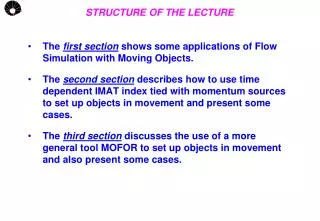
STRUCTURE OF THE LECTURE • The first section shows some applications of Flow Simulation with Moving Objects. • The second section describes how to use time dependent IMAT index tied with momentum sources to set up objects in movement and present some cases. • The third section discusses the use of a more general tool MOFOR to set up objects in movement and also present some cases.
Few Applications Requiring Moving-Body-Simulation • It permits the simulation of flows induced by bodies in motion. • Positive-displacement pumps and compressors of: piston-in-cylinder, rotating-vane, contra-rotating-helix, and • crank/connecting-rod/piston mechanisms in gasoline, diesel and steam engines; valve motions in engines; fuel injectors • fans, blowers and other kinds of turbomachinery; • shock-absorbers; • Vessel’s stirrers in chemical reactors; • parachute deployment; thrust-reversal devices in jet engines; • air-bags in automobiles; • trains entering, or passing in, tunnels; • any object/person/equipment falling from air into water.
FLOW SIMULATION WITH MOVING OBJECTS • The main sources of information are in: • Moving Bodies – Various Techniques Sec. 3-10 of In-Form report • MOFOR – Moving Frames Of Reference entry in POLIS • MOFOR – Cases and Tutorials • PHOENICS Library has some useful entries, check them out
TECHNIQUES TO REPRESENT THE MOVEMENT OF A BODY • There are two effective way to introduce the movement of a body: • Changing with time the distribution of the material-property indicator IMAT within the domain of study; and introducing momentum sources which are active only where IMAT has specific values. These two procedures ensure that these sources cause the fluid to move locally in accordance with the motion of the body. These procedures are described on the 2nd section of this lecture. • The MOFOR technique for describing the motion of objects, whether described by facets or formulae. It will be discussed in greater detail at the 3rd section of this lecture.
Exploring Technique #1:time dependent IMAT index tied with momentum sources (old fashion way) Two workshops will be developed using technique #1. They are quite simple cases derived from the phoenics’ library. The user is strongly recommended to look up at the available library cases.
wksh_mov_#1 • The whsk_mov_#1 is a (XY) flow field generated by the displacement of a blockage along the x direction inside a closed rectangular box. The figure below depicts the velocity field. • This scenario is likely to occur in damper such as the one employed in automobiles.
Defining the Domain NZ=1 & ZWLAST=0,1m NY=33 & YVLAST=0,6m NX=20 & XULAST=1,0m • The time grid is defined as follow: TFIRST=0, TLAST=10s and LSTEP=10. Each time step corresponds to 1 sec. • The spatial sizes are defined on the figure. • Set the properties to water, material (67) • Activate the velocity solver and use LVEL for turbulence modeling. • The boundaries are walls defined as objects. Use the first cell as pressure relief.
Setting Preliminaries – GROUP 1 • It is useful in group 1 declare the blockage material and its velocity. It is done using the Inform as shown on the lines below: INFORM1BEGIN REAL(MAT); MAT =100. REAL(VEL); VEL = 0.05 INFORM1END • The variable MAT = 100 specify the Aluminum and VEL = 0.05 m/s is the solid X velocity. It is chosen such that VEL corresponds to one X grid spacing per second.
Storing Material Index (PRPS) – GROUP 7 INFORM7BEGIN (STORED OF PRPS IS 67) DO II = 1,10 PATCH(TIME=:II:,CELL,:II:+4,:II:+4,11,23,1,NZ,:II:,:II:) (STORED OF PRPS AT TIME=:II: IS :MAT:) ENDDO • INFORM7END The first statement sets PRPS to the IMAT value of water throughout the domain; but the value is changed below for the cells occupied by the paddle Cells. They are marked by setting the value of PRPS in them to 100. The patch command is special because it changes accordingly to the DO loop. The counting variable :II: and also labels the arguments of the the patch command: PATCH(TIME=1,CELL,5,5,11,23,1,NZ,1,1) PATCH(TIME=2,CELL,6,6,11,23,1,NZ,2,2) ... PATCH(TIME=10,CELL,15,15,11,23,1,NZ,10,10) Notice the DO loop advances the patch in X direction as the time increases from 1 to 10. The following line store the material index accordingly to the patch name. This way defines as the solid blockage advances in space and in time.
Defining Properties – GROUP 9 INFORM9BEGIN (PROPERTY RHO1 IS 998) (PROPERTY VISL IS 1E-06) INFORM9END • It is still necessary define the liquid properties using Inform9 statements otherwise one won’t get the right results. • It must be a bug of version 3.5.1 because once you set PRPS = 67 in group 7 it would not require further property definition!
Defining X-Momentum Sources – GROUP 13 INFORM13BEGIN PATCH(I,CELL,1,NX,1,NY,1,NZ,1,10) (SOURCE of U1 at I is 0.05 with IMAT>=100!fixv) (A) (SOURCE of U1 at I is 1.E3*(VEL-U1) with IMAT>=100!LINE) (B) INFORM13END The patch command specify the whole domain from with time steps changing from 1 to 10. There are two options to set the momentum source on U1 equation: option (A) or (B). The user should choose one at a time: either (A) or (B). (A) sets U1 = 0.05 at patch I only at cells with imat>=100 using fixv (fixval). (B) sets U1 = 0.05 linearizing the source. Notice the 1E3 is a big number. This multiplier is a coefficient with causes, at the first iterations, U1 be equal to VEL, but at the converged solution this source will desapear because vel=u1. This procedure is more recommended because it helps to get the converged solution.
The Pressure and Vector Fields • Click here to open a movie_file displaying the pressure and vector field • This workshop’s Q1 is available for download : whsk_mov_#1.q1
wksh_mov_#2 • The whsk_mov_#2 is a (XY) flow field generated by turning a blockage in 90 degrees steps along the z direction inside a closed square box. The figure below depicts the velocity field. • This scenario is likely to occur near impeller blades used in mixing tanks.
Defining the Domain NZ=1 & ZWLAST=0,1m NY=21 & YVLAST=1,0m NX=21 & XULAST=1,0m • The time grid is defined as follow: TFIRST=0, TLAST=20s and LSTEP=20. • The dimensions are defined on the figure. • Set the properties to water, material (67) • Activate the velocity solver and use LVEL for turbulence modeling. • The boundaries are walls defined as objects. Use the first cell as pressure relief.
Setting Preliminaries – GROUP 1 • It is useful in group 1 declare the blockage material and its velocity. It is done using the Inform as shown on the lines below: INFORM1BEGIN REAL(MAT); MAT=100 REAL(OM); OM=1.571 REAL(YIC); YIC=0.5 REAL(XIC); XIC=0.5 INFORM1END • The variable MAT = 100 specify the Aluminum and OM = 0.784 rad/s is the solid angular Z velocity. YIC and XIC are the coordinates of the rotating axis where the pad revolves.
Storing Material Index (PRPS) – GROUP 7 INFORM7BEGIN (STORED OF PRPS IS 67) DO II = 1,19,2 PATCH(TIME1=:II:,CELL,11,11,8,14,1,NZ,II,II) (STORED OF PRPS AT TIME1=:II: IS :MAT:) ENDDO DO II = 2,20,2 PATCH(TIME2=:II:,CELL,8,14,11,11,1,NZ,:II:,:II:) (STORED OF PRPS AT TIME2=:II: IS :MAT:) ENDDO INFORM7END The blockage is 7 C.V. long and displaces in 90 degrees steps, that is, it is positioned along either the vertical or the horizontal. The blockage starts at the vertical position (aligned Y axis). The first DO loop specifies the vertical positions in time and the second DO does the horizontal positions. The DO loops count in odd and even steps and altogether define the blockage positioning along the time steps 1 thru 20
Defining Properties – GROUP 9 INFORM9BEGIN (PROPERTY RHO1 IS 998) (PROPERTY VISL IS 1E-06) INFORM9END • It is still necessary define the liquid properties using Inform9 statements otherwise one won’t get the right results. • It must be a bug of version 3.5.1 because once you set PRPS = 67 in group 7 it would not require further property definition!
Defining X- Y Momentum Sources – GROUP 13 INFORM13BEGIN PATCH(E1,EAST,1,NX,1,NY,1,NZ,1,LSTEP) (SOURCE OF U1 AT E1 IS VEL*(YG-YIC) WITH IMAT>=100!FIXV) (A) (SOURCE OF U1 AT E1 IS 1E+3*(VEL*(YG-YIC)-U1) WITH IMAT>=100!LINE) (B) PATCH(N1,NORTH,1,NX,1,NY,1,NZ,1,LSTEP) (SOURCE OF V1 AT N1 IS VEL*(XIC-XG) WITH IMAT>=100!FIXV) (A) (SOURCE OF V1 AT N1 IS 1E+3*(VEL*(XIC-XG)-V1) WITH IMAT>=100!LINE) (B) INFORM13END Likewise wksh_mov_#1 there are two options to set the momentum sources: (A) and (B). The later is preferred due to linear coupling with the solved velocities. The above statements make the vertical and horizontal velocities proportional to the corresponding distances from the paddle axis. They signify that, over the patch indicated, both x-direction first-phase velocity U1 and y-direction first-phase velocity V1 experience sources. The proportionality constant is large, which causes U1 to be close to the latter value when the equations have been solved. Similar remarks are appropriate to the V1 source.
The Pressure and Vector Fields • Click here to open a movie_file displaying the pressure and vector field • This workshop’s Q1 is available for download : whsk_mov_#2.q1
Exploring Technique #2:This workshop employs the so-called MOFORtechnique for describing the motion of objects. A series of 7 workshops will be used to introduce some of the main features of MOFOR technique. The user is strongly recommended to look up at the available library cases to enlarge the knowledge on MOFOR.
The MOFOR • The movement of an object is described by means of a formula employing the MOFOR technique. • It acts by moving, through the fixed computational grid, momentum sources to ensure that the velocities at locations within the body have the values implied by the prescribed motion. • It is far more simpler and powerful than technique #1 because it ties the movement to an object, that is, a multi-faceted shape which can be complex or not.
The translation and rotation of an object • A single method is used for describing its position and orientation relative to the reference frame (i.e. grid) which is being used to describe the CFD cells. It is described in terms of the 'bounding - box' concept: • The displacement of an object, which not deforms as it displaces, can be described by its translation and rotation in regard to the origin of the CFD-grid. • The position of the object in the CFD-grid space begins by stating the three numbers which define the position of the object's origin relative to the origin of the CFD-grid and three further numbers which signify the rotations which it has undergone. These rotations are sometimes called the Euler angles.
Articulated objects: the MOF format • Were all objects to move independently of one another, motion could be described by listing the values of the three translations and three rotations of the object's reference frame at successive instants of time. • However, many objects are connected together so that the movement of one enforces some movement of the another. Such objects are here called articulated. • A mechanical example is the crank/connecting-rod/piston trio.
Articulated objects: the MOF format • A human being, whose limbs are connected at joints (elbow, knee, etc) is also articulated. • It is this connectedness that the MOF format expresses by way of a hierarchy, whereby: • the torso (say) is regarded as the "root" element; • the upper arms are subservient to it, but have certain degrees of freedom (called "channels" for an unclear reason) relative to it; • the lower arm is subservient to the upper, but can move independently so far as the elbow allows; • the hand is subservient to the lower arm, because it must remain joined at the wrist; • the fingers.... and so to the fingertips.
Articulated objects: the MOF format • The MOF data file which describes a set of connected objects therefore has to convey information about the hierarchy (what is connected to what) and about the offset of each dependent element (also called "child") from its next-superior in the hierarchy (also called "parent"). • It also indicates in what way each object can move. • Finally it states, for a succession of times, what have been the movements in each of the degrees of freedom.
Describing the motion; • The information about the motion is conveyed in this 'MOF file‘. • This file is read by EARTH; and the information is placed in the appropriate locations in memory, at the start of the run. • Alternatively, the information is supplied to the same locations by way of In-Form formulae, expressed via SPEDATs and conveyed via EARDAT. • It should be clearly understood that the time steps used in the CFD calculation are not necessarily the same as those in the MOF description. They may be larger or smaller. • The necessary interpolation is performed inside EARTH.
Effects on the fluid: velocity • It is necessary to convey to the solver module that the velocity at velocity-grid nodes lying within the moving object is that prescribed, through the MOF file or the In-Form formulae, for that location. This is performed by introducing appropriate momentum sources at the relevant nodes. • It is of course necessary to determine, for each time step, which cells are inside which body, because more than one moving body may be present. The necessary coding for this exists inside EARTH. It requires no user intervention.
What are the necessary steps to set up a case using MOFOR • Have a MOFfile describing the object movement, • Using the VR editor, define the space and time grid, domain properties, activate the velocity solution and the boundary conditions and all objects required. • Write in Group 7, STORE(PRPS) • At the initialization make FIINIT PRPS equals to the domain material; • For the moving object make sure to select: a) object does not affect the grid and the b) object material is the domain material. • Finally at the output do not forget to damp the intermediate phi files.
Basics of MOF dataset format • MOF format has two-part structure designed for two classes of the attributes: HIERARCHY and MOTION, time dependent, data.
Basics of HIERARCHY in MOF dataset format (sample) • The word HIERARCHY at the top of the file is mandatory. It opens the hierarchy part of the attribute settings. UNITS is the word used to specify the attribute units - the default units are inches. METRES must be uppercase. • ROOT, JOINT and End Site are all key words of declaring the frames of reference of object-related coordinate systems. Each frame has a name; ROOT and JOINT must be uppercases and for internal storage reasons each joint's name is restricted to 16 characters. • ROOT is usually used to declare the origin of CFD-grid space. It is often followed by the number of subservient ROOTs or/and JOINTs within brackets. • Each JOINT is followed by a definition section consisting of an open bracket to a matching close bracket. Any joints defined inside the upper, superior joint are the children of this joint. The definition is usually of 1 or 2 lines - OFFSET and CHANNELs - plus any child joints. • The OFFSET is the position of the origin of the rotation axis relative to its parent. • The CHANNELS are the degrees of freedom. They define what type(s) of time dependent data are defined for this joint; the joint may translate or rotate or both, about any axis. • The End Site is the key words used to identify the end of the moving joint.
Basics of MOTION in MOF dataset format (sample) • MOTION is a mandatory key word. It identifies the beginning of the time dependent part of the MOF file. • FRAMES: They are the numbers of time moments at which data are given. The number of Frames may be bigger or smaller than the number of time steps of PHOENICS, but they are all equal in size. • Frame Time: is the time separation of each set of data. • For obvious reasons the total time of the particular set of data is equal to (Frames-1)*Frame Time. • There follows the numbers of frames sets of data; the number of values per line are defined by CHANNELS for each ROOT and JOINT objects as hierarchy specifies. • In what follows the number of MOF files will be exemplified and explained in details.
MOFOR Workshop’s Sequence • The workshops explore the MOFOR capabilities. It employs a single Q1 file with a moving plate. A sequence of 7 distinct MOF files explores the linear and rotating plate movements: • linear movement with uniform velocity • linear movement with accelerating and decelerating velocity • linear movement with oscillatory displacement • rotating movement • rolling movement (turning plus displacing) • flapping: rotating movement with oscillation • Twin flapping • The first case shows how to set up a q1 file to work with the mof file.
wksh_MOV1 • Let’s redo whsk_mov_#1 using MOFOR. The problem is a (XY) flow field generated by the displacement of a plate along the x direction inside a closed rectangular box. The figure below depicts the velocity field just for reference.
Defining the Domain NZ=1 & ZWLAST=0,1m NY=32 & YVLAST=0,6m NX=20 & XULAST=1,0m • The time grid is defined as follow: TFIRST=0, TLAST=10s and LSTEP=10. Each time step corresponds to 1 sec. • The spatial sizes are defined on the figure. • Set the properties to water, material (67) • Activate the velocity solver and use the Laminar flow model • The boundaries are walls defined as objects. Use the first cell as pressure relief.
Inserting the Moving Object • Name the block as PLATE • Set the PLATE origin and size as: (XYZ) (0.250, 0.200, 0.00) and (XYZ) (0.050, 0.218, 0.10) respectively. • The geometry pick from cube shape • Set: object does not affect the grid • Choose: The object’s material is the same of the domain properties. • Make the initialization FIINIT(PRPS) = 67 • At output select field dumping frequency equals to 1, and name the intermediate dump files as T • This q1 file will be used along the whole sequence. It is convenient to save it now. For convenience it is available for download here: MOFOR_BASIC.Q1
The MOF file HIERARCHY UNITS METRES ROOT Cham -> Defines the origin of the CFD-grip { JOINT PLATE -> Plate is the name of the moving object { CHANNELS 1 Xposition -> There is just one degree of freedom End Site } } MOTION Frames: 2 Frame Time: 10. -> The object takes 10 sec to travel from 0 to 0.5 m 0. 0.5 For convenience it is available to download: 1.MOF
Tying the MOF file with the Q1 file • The MOF file is tied to the Q1 file by declaring: SPEDAT(SET,MOFOR,MOFFILE,C,7.MOF)in Q1 group 19 or through the VR Editor within the SOURCES menu. At the entry MOFOR set it to ON and select a MOF file. • The MOF file name has to have 5 characters long. • It can be placed in any directory. • The results are pretty much the same the ones get in wksh_mov_#1. For reference the Q1 file to download is available: MOV1
wksh_MOV2 - Linear Acceleration • The objective is to displace linearly the object PLATE as: • Recalling the total time is 10 seconds, PLATE displacement is 0.6 meter. The figure below shows the displacement, the velocity and the acceleration • The
You do not have to change any line in the Q1 file, use the same from wksh_MOV1. • You have to work only at the MOTION section of theMOF file. • Set Frames: 11 and Frame Time: 1 so (Frames-1)*Frame Time = 10 sec. • Create 11 displacements starting from zero • For reference the Q1 and MOF files are available for download: MOV2.q1 and 2.MOF
wksh_MOV3 – Back & Forth • The objective is to displace forward and backward the object PLATE. • During the first 5 seconds the PLATE displaces 0.5 meters from its initial position. • It then displaces backwards so that after another 5 seconds it is again at its initial position. • You do not have to change any line in the Q1 file, use the same from wksh_MOV1. • You have to work only at the MOTION section of theMOF file. Set carefully the Frames and Frame Time. • For reference the Q1 and MOF files are available for download: MOV3.q1 and 3.MOF • The
wksh_MOV4 – Rotating Plate • The objective is to rotate 720 degrees the object PLATE during 10 seconds of simulation. • Inspect sample file and write your MOF file for this case. • You do not have to change any line in the Q1 file, use the same from wksh_MOV1. Although make sure your object origin and the offset statements on the mof file are compatible. • You also have to work at the MOTION section of theMOF file. Set carefully the Frames and Frame Time. • For reference the Q1 and MOF files are available for download: MOV4.q1 and 4.MOF • The
wksh_MOV5 – Rotating Plate • The objective is to rotate 720 degrees the object PLATE as it displaces 0.6 m during 10 seconds of simulation. • Inspect sample file and write your MOF file for this case. • You do not have to change any line in the Q1 file, use the same from wksh_MOV1. Although make sure your object origin and the offset statements on the mof file are compatible. • You also have to work at the HIERARCHY and MOTION sections of the MOF file. • For reference the Q1 and MOF files are available for download: MOV5.q1 and 5.MOF • The
wksh_MOV6 – Turning Plate • The objective is to oscillate from +45 to – 45 degrees the object PLATE during 10 seconds of simulation. • Inspect sample file and write your MOF file for this case. • You do not have to change any line in the Q1 file, use the same from wksh_MOV1. Although make sure your object origin and the offset statements on the mof file are compatible. • You also have to work at the MOTION section of theMOF file. Set carefully the Frames and Frame Time. • For reference the Q1 and MOF files are available for download: MOV6.q1 and 6.MOF • The file:///C:/phoenics/D_POLIS/D_WKSHP/mofor/MOF/LEARNMOF.HTM#4.4
wksh_MOV7 – Flapping Twin Plates • The objective is to oscillate anti-symmetrically two object PLATES from +45 to – 45 degrees during 10 seconds of simulation. • Inspect sample file and write your MOF file for this case. • For reference the Q1 and MOF files are available for download: MOV7.q1 and 7.MOF • The file:///C:/phoenics/D_POLIS/D_WKSHP/mofor/MOF/LEARNMOF.HTM#4.4
Closing Remarks • The MOFOR technique is still in development by CHAM team. • This series of workshop was prepared using phoenics v3.5. • The MOFOR show a bug when rotating frames were employed simultaneously with turbulence model LVEL. • One may try to activate LVEL model in cases 4 thru 7 and will get an error message in result file: it is missing material (0) the air. • There is no apparent reason for that. The message also suggest to insert in q1 the command line: SPEDAT(SET,MATERIAL,0,L,T), in doing this the program runs but I am not sure if the results are reliable or not!