Spatial Data Structure: Quadtree, Octree,and BSP tree
Spatial Data Structure: Quadtree, Octree,and BSP tree. Mengxia Zhu Fall 2007. Hierarchical structure. Data usually contains coherent regions of cells with similar properties hierarchical spatial enumeration encode the coherence in the volume data.


Spatial Data Structure: Quadtree, Octree,and BSP tree
E N D
Presentation Transcript
Spatial Data Structure: Quadtree, Octree,and BSP tree Mengxia Zhu Fall 2007
Hierarchical structure • Data usually contains coherent regions of cells with similar properties • hierarchical spatial enumeration encode the coherence in the volume data. • Is actually nothing more then a data structure built by recursive subdivision. • if a parent is not important then it's children aren't either.
Efficient storage of 2D data Completely non-important regions are represented by one cell; recursive subdivision done on others Quadtrees
Counterpart of Quadtree in 3D Each node has eight children instead of four Octrees
Recursive function for empty region construction: Recursive Subdivision for m=1,2….M
Case study: quad-tree in ray casting Also, in isosurface extraction. Min and Max value range
Hidden Surface Removal (HSR) • Why might a polygon be invisible? • outside the field of view • backfacing • occluded by object(s) closer to the viewpoint • we want to avoid spending time on these invisible polygons
Most objects are opaque. Avoid drawing any portion of an object that lies behind an opaque object, as seen from the camera’s point of view. Back-face removal algorithm: polygons whose normals point away from the camera are always occluded There is only a single object, and can fail if the object is not convex. Reduces by about half the number of polygons to be considered for each pixel. Every front-facing polygon must have a corresponding rear-facing one Back-Face Culling
For a scene consists of a sequence of intersecting objects. Correct occlusion relationship is required in order to render correct image. Occlusion
Draw polygons as an oil painter might: The farthest one first. Render the object from the back to front. Problem arise when no explicit visibility order can be found by forming a relationship cycle. Painter’s algorithm
Binary Space Partition Trees • BSP tree: traversed in a systematic way to draw the scene with HSR • Preprocess: organize all of polygons (hence partition)into a binary tree data structure • Runtime: correctly traversing this tree enumerates objects from back to front • Idea: divide space recursively into half-spaces by choosing splitting planes • Splitting planes can be arbitrarily oriented
BSP • Arbitrary plane split the space into two half-spaces: • Outside: the side pointed to by the outward-pointing normal to the plan • Inside: the other half-space Inside ones Outside ones
Rendering BSP Trees • RenderBSP(BSPtree *T) • BSPtree *near, *far; • if (T is a leaf node) • RenderObject(T) • if (eye on inside side of T->plane) • near = T->left; far = T->right; • else • near = T->right; far = T->left; • RenderBSP(far); • RenderBSP(near);
BSP Tree Construction • Split along the space defined by any plane • Classify all polygons into left or right half-space of the plane • If a polygon intersects plane, split polygon into two and classify them both • Recurse down the left half-space • Recurse down the right half-space
Discussion: BSP Tree Cons • No bunnies were harmed in previous example • But what if a splitting plane passes through an object? • Split the object; give half to each node Ouch
Summary: BSP Trees • Pros: • Preprocess done once • Only writes to framebuffer (no reads to see if current polygon is in front of previously rendered polygon, i.e., painters algorithm) • Cons: • Computationally intense preprocess stage • Slow time to construct tree • Splitting increases polygon count
The Z-Buffer Algorithm • Both BSP trees and Warnock’s algorithm (subdivide primitive into viewports in a recursive way) were proposed when memory was expensive • Example: first 512x512 framebuffer > $50,000! • Ed Catmull (mid-70s) proposed a radical new approach called z-buffering. • The big idea: resolve visibility independently at each pixel
The Z-Buffer Algorithm • We know how to rasterize polygons into an image discretized into pixels:
The Z-Buffer Algorithm • What happens if multiple primitives occupy the same pixel on the screen? Which is allowed to paint the pixel?
The Z-Buffer Algorithm • Idea: retain depth (Z in eye coordinates) through projection transform • Use canonical viewing volumes • Each vertex has z coordinate (relative to eye point) intact
The Z-Buffer Algorithm • Augment framebuffer with Z-buffer or depth buffer which stores Z value at each pixel • At frame beginning, initialize all pixel depths to • When rasterizing, interpolate depth (Z) across polygon and store in pixel of Z-buffer • Suppress writing to a pixel if its Z value is more distant than the Z value already stored there
Interpolating Z • Edge equations: Z is just another planar parameter: z = (-D - Ax – By) / C If walking across scanline by (Dx) znew = zold – (A/C)(Dx) • Look familiar? • Total cost: • 1 more parameter to increment in inner loop • 3x3 matrix multiply for setup • Edge walking: just interpolate Z along edges and across spans
Z-Buffer Pros • Simple!!! • Easy to implement in hardware • Polygons can be processed in arbitrary order • Easily handles polygon interpenetration • Enables deferred shading • Rasterize shading parameters (e.g., surface normal) and only shade final visible fragments
Z-Buffer Cons • Lots of memory (e.g. 1280x1024x32 bits) • With 16 bits cannot discern millimeter differences in objects at 1 km distance • Read-Modify-Write in inner loop requires fast memory • Hard to do analytic antialiasing • We don’t know which polygon to map pixel back to • Hard to simulate translucent polygons • We throw away color of polygons behind closest one
Reference • Slides from David Brogan at University of Virginia