
Finite State Machines 2
E N D
Presentation Transcript
Finite State Machines 2 95-771 Data Structures and Algorithms for Information Processing 95-771 Data Structures and Algorithms for Information Processing
Deterministic Finite-State Automata (review) • A DFSA can be formally defined as A = (Q, , , q0, F): • Q, a finite set of states. • , a finite alphabet of input symbols. • q0 Q, an initial start state. • F Q, a set of final states. • (delta): Q x Q, a transition function. 95-771 Data Structures and Algorithms for Information Processing
We can define on words, w, by using a recursive definition: • w : Q x * Q A function of (state, word) to a state. • w(q,) = q If in state q, output state q if word is . • w(q,xa) = (w(q,x),a) Otherwise, use for one step and recurse. 95-771 Data Structures and Algorithms for Information Processing
For an automaton A, we can define the language of A: • L(A) = {w* : w(q0,w) F } • L(A) is a subset of all words w of finite length over , such that the transition function w(q0,w) produces a state in the set of final states (F). • Intuitively, if we think of the automaton as a graph structure, then the words in L(A) represent the “paths” which end in a final state. If we concatenate the labels from the edges in each such path, we derive a string w L(A). 95-771 Data Structures and Algorithms for Information Processing
Regular Languages A language L * is called a regular languageif there exists a finite-state automaton, A, such that L = L(A). Examples of regular languages: L = * (all finite words in ) L = (the empty set) L = {} (set containing just the empty string) (As a self-test, draw a DFSA, A, for each L, such that L = L(A). Use = {a,b,c}.) 95-771 Data Structures and Algorithms for Information Processing
Digression: Encoding a DFA • Number of states. • First on 0. • First on 1. • Second on 0. • Second on 1. • Accepting states. 0 1 2 0 1 1 0010010101001100 Quiz: Does every Java program have an encoding? Is every possible Java program found in {0,1}* ? 95-771 Data Structures and Algorithms for Information Processing
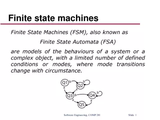
Non-Deterministic Finite-State Automata (NDFSA) The DFSA we have studied so far are called deterministic, because for any given word w there is a single path through the automaton (or, more formally, w(q0,w) = qn; the automaton transitions to a single state on any given word). The result is “well-determined” because it can have only a single value. 95-771 Data Structures and Algorithms for Information Processing
NDFSA We can extend the definition of DFSA to be less restrictive, such that output of the transition function is a set of states rather than a single state: : Q x 2Q The non-deterministic can produce as output any subset of Q, so in the definition we use 2Q to indicate the power set(set of all possible subsets) of Q. Will this change add power? 95-771 Data Structures and Algorithms for Information Processing
Since there can be more than one “path” through an NDFSA for a given word w, we have to revise our notion of acceptance for NDFSA. An NDFSA accepts a word w if there exists some computation path that ends in a final state q F. 95-771 Data Structures and Algorithms for Information Processing
NDFSA Example 95-771 Data Structures and Algorithms for Information Processing
NDFSA Note the following non-deterministic transitions: (q0,0) = {q0,q3} (q0,1) = {q0,q1} (As a self-test, trace all of the paths through the example NDFSA for w = 0100. Indicate each path by writing down the sequence of states.) 95-771 Data Structures and Algorithms for Information Processing
For NDFSA, we can expand the notion of on letters to on words, w, by using a recursive definition similar to the one we used for DFSA: • w : Q x * 2Q • w(q,) = {q} • w(q,xa) = {p | for some state r w(q,x), p (r,a)} • The third statement indicates that: starting in state q, and reading the string x, followed by the symbol a, we can be in state p, if and only if one possible state we can be in after reading x is r, and from r we may go to p upon reading a. 95-771 Data Structures and Algorithms for Information Processing
We can also define a transition function that accepts a set of states as one of its inputs: P : 2Q x * 2Q So, if P Q, then P(P,w) = Uq in Pw(q,w). Restated in English: If P is a subset of the states in Q, then the value of the transition function P on P and some word w will be the union of all of the sets of states produced by computing w(q,w) for every q in P. For example, in the automaton shown above, P({q1,q3},1) = {q2}. The transition function on sets of states allows us to compute all possible next states after each symbol or word is encountered, giving the effect of trying all paths in parallel. 95-771 Data Structures and Algorithms for Information Processing
Equivalence of NDFSA and DFSA The set of languages L(A) for all NDFSA is also the set of regular languages. For every NDFSA A, we can construct an equivalent DFSA B such that L(A) = L(B). The equivalence is achieved by using a single state in the DFSA to represent a set of states in the NDFSA. The DFSA keeps track of all possible states that the NDFSA could be in after reading the same input. Formally, if the NDFSA has a set of states Q, then the equivalent DFSA has a set of states Q’ = 2Q (all possible subsets of Q). 95-771 Data Structures and Algorithms for Information Processing
An element of Q’ is denoted as [q1,q2,…,qm]. q’0 = [q0]. Then we can define ’([q1,q2,…,qm],a) = [p1,p2,…,pn] if and only if P({q1,q2,…,qm},a) = {p1,p2,…,pn}. 95-771 Data Structures and Algorithms for Information Processing
Example Conversion of NDFSA to DFSA 95-771 Data Structures and Algorithms for Information Processing
We can construct an equivalent DFSA, A’ = {Q,{0,1},’,[q0],F) such that L(A’) = L(A), as follows. The elements of Q will be the power set of {q0,q1}, represented using the square bracket notation introduced in the previous section to indicate that each state in Q represents a set of states in the original NDFSA. Here is the set of states in Q: [q0], [q1], [q0,q1], 95-771 Data Structures and Algorithms for Information Processing
NDFSA to DFSA 95-771 Data Structures and Algorithms for Information Processing
Then we must define the transitions from[q0,q1]: ’([q0,q1],0) = [q0,q1], since ({q0,q1},0) = (q0,0) U (q1,0) = {q0,q1} U = {q0,q1}; ’([q0,q1],1) = [q0,q1], since ({q0,q1},1) = (q0,1) U (q1,1) = {q1} U {q0,q1} = {q0,q1}. The set F of final states is the set of all states in Q that contain the original final state, q1; so F = {[q1],[q0,q1]}. (As a self-test, trace the computation of some sample strings through both the NDFSA and the equivalent DFSA in order to convince yourself that they really are equivalent. Try the conversion yourself for another small NDFSA.) 95-771 Data Structures and Algorithms for Information Processing
Context-Free Grammars and Context-Free Languages • A context-free grammar G is defined formally as: • V: a finite set of variables (“non-terminals”); e.g., A, B, C, … • T: a finite set of symbols (“terminals”), e.g., a, b, c, … • P: a set of production rules of the form A , where A V and (V U T)* • S: a start non-terminal; S V • Production rules can also be thought of as derivations. 95-771 Data Structures and Algorithms for Information Processing
Assume G = ({A},{a,b},{A aAb, A }, A) Note that L(G) = {,ab,aabb,aaabbb,…}. We can derive each string in L(G) by using the two production rules to rewrite the initial expression, which consists of just the start symbol. For example, the derivation of aabb: A aAb (apply first rule) aaAbb (apply first rule) aabb (apply second rule) 95-771 Data Structures and Algorithms for Information Processing
We use the symbol to indicate that a derivation exists from an expression to another expression for a given grammar; e.g., for the grammar G defined above, A aabb. Then we can define L(G) as follows: L(G) = { w T* | S w } In plain English, the language of a grammar G is the set of all strings that can be derived from the start symbol S using the production rules in P. A language L is a context-free language if there exists a grammar G such that L = L(G). 95-771 Data Structures and Algorithms for Information Processing
Context-Free Language vs. Regular Languages • Consider the grammar we specified in a prior example. A closed-form expression for this grammar is: L(G) = {anbn | n 1} • Question: Why is L(G) not a regular language? Recall the definition of a regular language. For every regular language L, there exists some DFSA A such that L(A) = L. Why isn’t it possible to define a DFSA which accepts L(G) = {anbn | n 1}? 95-771 Data Structures and Algorithms for Information Processing
Answer: Because the derivation of each w L(G) adds exactly one a and one b to the word being constructed, each time the first production is fired. A DFSA can accept only one symbol at a time, and it cannot “remember” how many instances of a particular symbol it has seen. Any DFSA we define that accepts strings of the form {anbn | n 1} would also accept other strings {ambn | m n}. By the pigeon hole principle, n+1 a’s will require that an n state machine be in some same state more than once. (Self-test: try to construct a DFSA that accepts precisely {anbn | n 1}, to convince yourself that this is the case.) 95-771 Data Structures and Algorithms for Information Processing
Pushdown Automata In the previous lecture, we explained how a DFSA is used to recognize (accept strings in) regular languages. Context-free languages also have a machine counterpart: the pushdown automata (PDA). To recognize context-free languages, we need to define a machine that solves the “memory problem” we noted above. The solution comes from adding a stack data structure to a finite-state machine. 95-771 Data Structures and Algorithms for Information Processing
To understand how the stack is used in conjunction with a finite-state machine, let’s visualize a pushdown automaton for our example context-free language, L(G) = {anbn | n 1}. • Let’s define a machine with two states, as follows: • When the machine is in q0 : If an a is read, push a marker on the stack and stay in q0; if a b is read and there is a marker on the stack, pop the stack and go to q1. • When the machine is in q1: If a b is read and there is a marker on the stack, pop the stack and stay in q1. • Assume that all other transitions are undefined and cause the machine to halt, rejecting the input. • The computation ends when both the input and the stack are empty. 95-771 Data Structures and Algorithms for Information Processing
Why does this machine accept L(G) = {anbn | n 1}? • In the start state q0, the only possible moves are a) read one or more a’s, adding a marker to the stack for each a which is seen; b) read exactly one b, popping the stack and moving to q1. • Assuming we have read n a’s and 1 b, then there will be n – 1 markers left on the stack. • In state q1, the only possible move is to read a b and pop the stack. • Since the machine will halt (and reject) if there is input remaining and the stack is empty, the only way to exhaust the input and end with an empty stack is to read exactly the same number of a’s and b’s. 95-771 Data Structures and Algorithms for Information Processing
Here’s the formal definition of a pushdown automaton: M = (Q,,,,q0,F) Q: a set of states : the alphabet of input symbols : the alphabet of stack symbols : Q x x Q x q0: the initial state F: the set of final states 95-771 Data Structures and Algorithms for Information Processing
Intuitively, if (q,s,) = (q’,), then M, whenever it is in state q with at the top of the stack, may read s from the input, replace by on the top of the stack, and enter state q’. Pushing, popping, and preserving the stack are possible: (q,a,) = (q’,A) push A on the stack without popping (q,a,A) = (q’,) pop A from the stack without pushing (q,a,) = (q’,) stack unchanged 95-771 Data Structures and Algorithms for Information Processing
Now we can define a PDA M, such that L(M) = L(G) = {anbn | n 1}: M = ({q0,q1},{a,b},{A},,q0,{q1}) (q0,a,) = (q0,A) (q0,b,A) = (q1,) (q1,b,A) = (q1,) (Self-test: Trace the operation of M on some strings in L(G), and some strings not in L(G). Assume computation is successful (accept) only if the input is empty, the stack is empty, and the machine is in final state q1.) (Self-test: Build a PDA that recognizes {0i1j2k: k = i * j} . Note: You will not be able to succeed. The pumping lemma can be used to prove this result.) 95-771 Data Structures and Algorithms for Information Processing