Statistical Classification
Statistical Classification. Rong Jin. X. Input. Y. Output. ?. Classification Problems. Given input X={ x 1 , x 2 , …, x m } Predict the class label y Y Y = {-1,1}, binary class classification problems Y = {1, 2, 3, …, c }, multiple class classification problems

Statistical Classification
E N D
Presentation Transcript
Statistical Classification Rong Jin
X Input Y Output ? Classification Problems • Given input X={x1, x2, …, xm} • Predict the class label y Y • Y = {-1,1}, binary class classification problems • Y = {1, 2, 3, …, c}, multiple class classification problems • Goal: need to learn the function: f: X Y
Examples of Classification Problem • Text categorization: • Input features X: • Word frequency • {(campaigning, 1), (democrats, 2), (basketball, 0), …} • Class label y: • Y = +1: ‘politics’ • Y = -1: ‘non-politics’ Politics Non-politics Doc: Months of campaigning and weeks of round-the-clock efforts in Iowa all came down to a final push Sunday, … Topic:
Examples of Classification Problem • Text categorization: • Input features X: • Word frequency • {(campaigning, 1), (democrats, 2), (basketball, 0), …} • Class label y: • Y = +1: ‘politics’ • Y = -1: ‘not-politics’ Politics Non-politics Doc: Months of campaigning and weeks of round-the-clock efforts in Iowa all came down to a final push Sunday, … Topic:
Examples of Classification Problem • Image Classification: • Input features X • Color histogram • {(red, 1004), (red, 23000), …} • Class label y • Y = +1: ‘bird image’ • Y = -1: ‘non-bird image’ Which images are birds, which are not?
Examples of Classification Problem • Image Classification: • Input features X • Color histogram • {(red, 1004), (blue, 23000), …} • Class label y • Y = +1: ‘bird image’ • Y = -1: ‘non-bird image’ Which images are birds, which are not?
X Input Y Output ? Doc: Months of campaigning and weeks of round-the-clock efforts in Iowa all came down to a final push Sunday, … f: image topic f: doc topic Birds Not-Birds Politics Not-politics Classification Problems How to obtain f ? Learn classification function f from examples
Learning from Examples • Training examples: • Identical Independent Distribution (i.i.d.) • Each training example is drawn independently from the identical source • Training examples are similar to testing examples
Learning from Examples • Training examples: • Identical Independent Distribution (i.i.d.) • Each training example is drawn independently from the identical source
Learning from Examples • Given training examples • Goal: learn a classification function f(x):XY that is consistent with training examples • What is the easiest way to do it ?
(k=4) (k=1) K Nearest Neighbor (kNN) Approach How many neighbors should we count ?
Cross Validation • Divide training examples into two sets • A training set (80%) and a validation set (20%) • Predict the class labels of the examples in the validation set by the examples in the training set • Choose the number of neighbors k that maximizes the classification accuracy
Leave-One-Out Method • For k = 1, 2, …, K • Err(k) = 0; • Randomly select a training data point and hide its class label • Using the remaining data and given K to predict the class label for the left data point • Err(k) = Err(k) + 1 if the predicted label is different from the true label • Repeat the procedure until all training examples are tested • Choose the k whose Err(k) is minimal
Leave-One-Out Method • For k = 1, 2, …, K • Err(k) = 0; • Randomly select a training data point and hide its class label • Using the remaining data and given K to predict the class label for the left data point • Err(k) = Err(k) + 1 if the predicted label is different from the true label • Repeat the procedure until all training examples are tested • Choose the k whose Err(k) is minimal
(k=1) Leave-One-Out Method • For k = 1, 2, …, K • Err(k) = 0; • Randomly select a training data point and hide its class label • Using the remaining data and given k to predict the class label for the left data point • Err(k) = Err(k) + 1 if the predicted label is different from the true label • Repeat the procedure until all training examples are tested • Choose the k whose Err(k) is minimal
(k=1) Leave-One-Out Method • For k = 1, 2, …, K • Err(k) = 0; • Randomly select a training data point and hide its class label • Using the remaining data and given k to predict the class label for the left data point • Err(k) = Err(k) + 1 if the predicted label is different from the true label • Repeat the procedure until all training examples are tested • Choose the k whose Err(k) is minimal Err(1) = 1
Leave-One-Out Method • For k = 1, 2, …, K • Err(k) = 0; • Randomly select a training data point and hide its class label • Using the remaining data and given k to predict the class label for the left data point • Err(k) = Err(k) + 1 if the predicted label is different from the true label • Repeat the procedure until all training examples are tested • Choose the k whose Err(k) is minimal Err(1) = 1
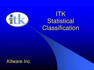
k = 2 Leave-One-Out Method • For k = 1, 2, …, K • Err(k) = 0; • Randomly select a training data point and hide its class label • Using the remaining data and given k to predict the class label for the left data point • Err(k) = Err(k) + 1 if the predicted label is different from the true label • Repeat the procedure until all training examples are tested • Choose the k whose Err(k) is minimal Err(1) = 3 Err(2) = 2 Err(3) = 6
Probabilistic interpretation of KNN • Estimate the probability density function Pr(y|x) around the location of x • Count of data points in class y in the neighborhood of x • Bias and variance tradeoff • A small neighborhood large variance unreliable estimation • A large neighborhood large bias inaccurate estimation
Weighted kNN • Weight the contribution of each close neighbor based on their distances • Weight function • Prediction
Estimate 2in the Weight Function • Leave one cross validation • Training dataset D is divided into two sets • Validation set • Training set • Compute the
Estimate 2in the Weight Function Pr(y|x1, D-1) is a function of 2
Estimate 2in the Weight Function Pr(y|x1, D-1) is a function of 2
Estimate 2in the Weight Function • In general, we can have expression for • Validation set • Training set • Estimate 2 by maximizing the likelihood
Estimate 2in the Weight Function • In general, we can have expression for • Validation set • Training set • Estimate 2 by maximizing the likelihood
Optimization • It is a DC (difference of two convex functions) function
Challenges in Optimization • Convex functions are easiest to be optimized • Single-mode functions are the second easiest • Multi-mode functions are difficult to be optimized
Gradient Ascent (cont’d) • Compute the derivative of l(λ), i.e., • Update λ How to decide the step size t?
Gradient Ascent: Line Search Excerpt from the slides by Steven Boyd
Gradient Ascent • Stop criterion • is predefined small value • Start λ=0, Define , , and • Compute • Choose step size t via backtracking line search • Update • Repeat till
Gradient Ascent • Stop criterion • is predefined small value • Start λ=0, Define , , and • Compute • Choose step size t via backtracking line search • Update • Repeat till
ML = Statistics + Optimization • Modeling Pr(y|x;) • is the parameter(s) involved in the model • Search for the best parameter • Maximum likelihood estimation • Construct a log-likelihood function l() • Search for the optimal solution
Instance-Based Learning (Ch. 8) • Key idea: just store all training examples • k Nearest neighbor: • Given query example , take vote among its k nearest neighbors (if discrete-valued target function) • take mean of f values of k nearest neighbors if real-valued target function
When to Consider Nearest Neighbor ? • Lots of training data • Less than 20 attributes per example • Advantages: • Training is very fast • Learn complex target functions • Don’t lose information • Disadvantages: • Slow at query time • Easily fooled by irrelevant attributes
KD Tree for NN Search • Each node contains • Children information • The tightest box that bounds all the data points within the node.
Curse of Dimensionality • Imagine instances described by 20 attributes, but only 2 are relevant to target function • Curse of dimensionality: nearest neighbor is easily mislead when high dimensional X • Consider N data points uniformly distributed in a p-dimensional unit ball centered at original. Consider the nn estimate at the original. The mean distance from the original to the closest data point is:
Curse of Dimensionality • Imagine instances described by 20 attributes, but only 2 are relevant to target function • Curse of dimensionality: nearest neighbor is easily mislead when high dimensional X • Consider N data points uniformly distributed in a p-dimensional unit ball centered at origin. Consider the nn estimate at the original. The mean distance from the origin to the closest data point is: