Download
1 / 22
220 likes | 534 Vues
. Dan Stefanoiu Associate Professor. Florin Ionescu Professor. . . The multiconference on Computational Engineering in Systems Applications. July 9-11, 2003, Lille, FRANCE. Maximum Verisimilitude Frequency Averaging of Signals. Danstef@fh-konstanz.de. Ionescu@fh-konstanz.de.

E N D
Dan StefanoiuAssociate Professor Florin IonescuProfessor The multiconference on Computational Engineering in Systems Applications July 9-11, 2003, Lille, FRANCE Maximum Verisimilitude Frequency Averaging of Signals Danstef@fh-konstanz.de Ionescu@fh-konstanz.de Dandusus@yahoo.com University of Applied Sciences, Konstanz, Germany www.fh-konstanz.de Department of Mechatronics # On leave from“Politehnica” University of Bucharest, Romania www.pub.ro Department of Automatic Control and Computer Science Research developed with the support of Alexander von Humboldt Foundation, Germany www.avh.de
Headlines • A data/signal (pre)processing paradigm • On Time Domain Synchronous Averaging (TDSA) • Noise hypotheses and Maximum Verisimilitude The Frequency Averaging Method (FAM) • Simulation results • Conclusion References 1
Is it possible to make a clear distinction between the util data and the noise? & Un-mix? Un-mix & How to extract the util data from a noisy signal? stationary data dominates the noise A data/signal (pre)processing paradigm Corrupting noise Noisy/fractal signal Util data non stationary noise dominates the data It might be a difficult Signal Processing problem. Usually, it is difficult, if not impossible. It depends tremendously on definition of “util” data. 2
How the “util” data can be defined ? Two properties are desirable: A data/signal (pre)processing paradigm • Partial or significant attenuation of noise such that the extracted signal carries almost the same information as the genuine one. • Partial or significant attenuation of redundancy such that the extracted signal encodes almost the same information but within a smaller number of data samples. Denoising Compressing Signal compaction Problems: • The rule of combination between the deterministic data and the stochastic noise is usually unknown. One uses the additive/superposition hypothesis (which can fail for difficult signals such as: seismic, underwater acoustic or celestial). Noise is modeled by using the Theorem of Central Limit. Parametric Non parametric Any acquired data are affected by a certain amount of Gaussian noise, usually white. • Even the combination between deterministic and stochastic components is known, how to separate them? Mathematical models are required. 3
3 classes of signal compaction models Time Frequency Time-frequency In time domain A data/signal (pre)processing paradigm Lagrange, Laguerre, Chebischev, Gauss, splines, etc. Interpolation models parametric Compacted data provided by re-sampling with a smaller sampling rate. Noise only weakly attenuated, because models are usually too fitted to data. based on experimental identification recipes Least Squares (LS) models parametric Models that fit the best to the data, not necessarily maximally. The more complex the model the better the compaction performance. Typical example: a time series Simple models are preferred in pre-processing. General trend (deterministic) • Polynomial, degree < 7 Seasonal component (deterministic) • Elementary harmonics Colored noise (stochastic) • Auto-regressive 4
3 classes of signal compaction models Time Frequency Time-frequency In time domain A data/signal (pre)processing paradigm based on Time Domain Synchronous Averaging Averaging models non-parametric Described later. In frequency domain based on spectral estimation techniques Spectral smoothing models non-parametric Smoothing the spectrum means removing some noise. In general, complex models and methods. Compacted signal difficult to provide because the spectrum looses the phase information. based on Maximum Verisimilitude DFT Averaging Averaging models parametric New Introduced within this presentation. In time-frequency domain Short Fourier Transform, Wavelet Transform, Wigner-Ville Transform, etc. Transformation models parametric Suitable for non stationary data sets (with spectrum variable in time). Complex models and methods rather inappropriate if only pre-processing is wanted. 5
number of periods (the bigger, the better) Originates from early works in Signal Processing, such as Welch method of spectral estimation(1967). Devised by P.D. McFadden in 1987. On Time Domain Synchronous Averaging (TDSA) TDSA like introduced by McFadden How can x be extracted from y? Measured data model Exploit the known periodicity. Idea harmonic signal with known/measurable period unknown noise (with null average) Util data model Time averaging of measured data Comb filter Dirac impulse Fourier Transform Slide the comb along the data and average only the samples pointed by its teeth. Comb rule 6
TDSA like introduced by McFadden Trmust accurately be known • Drawbacks On Time Domain Synchronous Averaging (TDSA) aNis not necessarily periodic, though x should be periodic Improved model of util data window extracting only N samples from measured data impulses train (ideal comb, uniform) Util data denoised and restricted to one period Signal compacted Generalized model of util data TDSA is simple and appealing for applications The comb rule works identically. localization instants of comb teeth synchronization signal (ideal comb, non necessarily uniform) the synchronization signal must accurately be known/acquired • Drawbacks the method is impractical for asynchronous signals (not necessarily periodic) 7
... ... Frequency effects of TDSA McFadden gave a frequency interpretation of TDSA by using the Continuous Fourier Transform after extending its definition to a train of impulses. On Time Domain Synchronous Averaging (TDSA) But: more naturally is to operate with discrete signals (as the measured data are) and the Discrete Fourier Transform (DFT). Direct Inverse DFTN General case sampling period Measured data number of samples per period Synchronization signal unit impulse Util data model 8 comb teeth localization instants
... ... Frequency effects of TDSA Theorem 1 On Time Domain Synchronous Averaging (TDSA) Algorithm | ... Step 1. Segment the data intoNsuccessive frameswithKssamples each, starting from each synchronization impulse. | Frame 3 | Frame 2 | Frame 1 Step 2. Compute the DFT of orderKsfor each frame. Step 3. Average the DFTs by using some harmonic weights. Frames may overlap. They do not overlap for uniform synchronization. • Interpretation If the main harmonic of signal has a constant period (Ks), their (N) DFTs are quite similar and thus, by averaging them, a noise reduction is expected. The synchronization signal plays a crucial role in averaging. Inappropriate synchronization leads to noise amplification. 9
Split the discrete spectrum of y into M non overlapped sub-bands with equal bandwidth and set . |DFTN| ... 0 1 2 M-1 0 H2 The noises Vm are white Gaussian with null mean and unknown variances . ... Measured data not necessarily periodic. Measured data model compacted signal with support unknown noise (hypotheses follow) Noise hypotheses and Maximum Verisimilitude Noise not necessarily additive. Hypotheses H1 The DFTN of signal y is affected by a set of M complex valued and additive sub-band noises Vm with finite supports included into corresponding sub-bands. Noises are orthogonal each other. Here is the DFT model of measured data: How can the deterministic models Am be extracted from Y? Here are the probability densities of noises: 10
parameters vector extended with unknown variance Idea Use the Maximum Verisimilitude Method (MVM). Example: polynomial Util data parametric model Noise hypotheses and Maximum Verisimilitude Linear, for simplicity. (measured) data vector of length pm parameters vector (of length pm) MVM optimization problems data segment in sub-band m stability domain of model density of conditional probability between data and parameters Parameters should be set such that the measured data occur withmaximum probability, i.e. withmaximum verisimilitude. Example: pm=0 simple averages of DFT data in sub-band m Theorem 2 (that solves the optimization problems) The nice properties of LS estimation are thus inherited. convergence accuracy of estimation (improves with K ) 11
operations How the MVM estimations can be employed to construct the compacted signal ? General solution Simple concatenation of MVM estimates gives the DFT estimation of denoised signal. The Frequency Averaging Method (FAM) • The resulted spectrum keeps the appearance of original spectrum, but is smoother. Compression is achieved by interpolation of MVM estimates in a smaller number of spectral lines, say L<K . Example: interpolation of polynomial model Frequency Averaging Algorithm 12
Advantages of FAM • No synchronization signal is required. The Frequency Averaging Method (FAM) • Data can be periodic or not. If data are periodic: it is not necessary to know the main period; if the period known, the number of interpolation spectral lines (L) can be set accordingly, to increase the accuracy; if the period is poorly estimated, the compacted signal will just lie inside a support that is not divisible by the period; • Non uniform splitting of signal bandwidth can lead to better results, especially when the signal energy is concentrated only inside certain sub-bands. • Drawbacks of FAM • More complex than TDSA, though the complexity can be controlled by the user. • Good accuracy is obtained for data sets which are large enough. This is the price paid for the absence of synchronization signal. • Parameters N, M and K should be set as a result of a trade-off. On one hand: accuracy is bigger for a bigger number of spectral lines per sub-band (K). On the other hand: the original spectrum is better “imitated” by the compacted one if the number of sub-bands is bigger (M), i.e. if the number of spectral lines per sub-band is smaller, given the number of samples (N). 13
operations (no interpolation is necessary) Consequences of FAM A procedure for SNR estimation The Frequency Averaging Method (FAM) Theorem 3 (simple frequency average models) Same comb rule. TDSA 14
Toy example: a sine wave sunk into Gaussian noise Simulation results SNR 6 dB ( 33% noise) Original signal and spectrum SNR 4.7 dB Compacted signal and spectrum for M=333 SNR 7.1 dB Compacted signal and spectrum for M=71 The SNR is not necessarily increasing for compacted signal. 15
Variation of SNR with the compacted support length of noisy sine wave Simulation results The trade-off between the data length and the number of sub-bands is important. 16
Noisy vibration (a) and spectra (b) provided by a bearing in service (B3850609) Simulation results Estimated SNR 3.27 dB variable rotation period due to a load and an incipient defect Estimated SNR 10.53 dB rotation period poorly estimated About 4 full rotations The spectral appearance of compacted signal is similar to the original one. 17
Filtered vibration (a) and spectra (b) provided by a bearing in service (B3850609) Simulation results Estimated SNR 5.72 dB Estimated SNR 12.38 dB this is an asynchronous signal About 4 full rotations of unfiltered vibration The spectrum of compacted signal still keeps the appearance of the original. 18
|DFTN| ... 0 1 2 M-1 0 ... ... ... How to extract the util data from a noisy signal? For example, with the help of Time Domain Synchronous Averaging, whenever a synchronization signal accompanies the measured data. Conclusion The Frequency Averaging Method based on maximum verisimilitude can be employed whenever the synchronization signal is missing or poorly estimated. Is it possible to make a clear distinction between the util data and the noise? Usually not, but it depends on how the concept of “util data” is defined. There always is a part of noise treated as util data and a part of util data removed together with noises. 19
References 1. Cohen L. Time-Frequency Analysis, Prentice Hall, New Jersey, USA, 1995. 2. Ionescu F., Arotaritei D. Fault Diagnosis of Bearings by Using Analysis of Vibrations and Neuro-Fuzzy Classification, Proceedings of ISMA’23 Conference, Leuven, Belgium, September 16-18, 1998. 3. McFadden P.D. A Revised Model for the Extraction of Periodic Waveforms by Time Domain Averaging, Mechanical Systems and Signal Processing, Vol. 1, No. 1, pp. 83-95,1987. 4. McFadden P.D. Interpolation Techniques for Time Domain Averaging of Gear Vibration, Mechanical Systems and Signal Processing, Vol. 3, No. 1, pp. 87-97,1989. 5. Oppenheim A.V., Schafer R. Digital Signal Processing, Prentice Hall, New York, USA, 1985. 6. Proakis J.G., Manolakis D.G. Digital Signal Processing. Principles, Algorithms and Applications., Prentice Hall, New Jersey, USA, 1996. 7. Söderström T., Stoica P. System Identification, Prentice Hall, London, UK, 1989. 8. Welch P.D. The Use of Fast Fourier Transform for the Estimation of Power Spectra: A Method Based on Time Averaging over Short Modified Periodograms, IEEE Transactions on Audio and Electroacoustics, Vol. AU-15, pp. 70-73, June 1967. 20
Bodensee & Säntis (2542 m) (Danny’s photo gallery) Thank you! Florin Ionescu Dan Stefanoiu • Dandusus@yahoo.com • Danstef@fh-konstanz.de • Ionescu@fh-konstanz.de • http://www.geocities.com/dandusus/Danny.html