Download
1 / 26
360 likes | 733 Vues
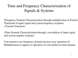
Time and Frequency Characterization of Signals & Systems. Frequency Domain Characterization through multiplication of Fourier Transform of input signal and system frequency response. ( Transfer Function). Time Domain Characterization through convolution of input signal

E N D
Time and Frequency Characterization of Signals & Systems • Frequency Domain Characterization through multiplication of Fourier • Transform of input signal and system frequency response. • ( Transfer Function). • Time Domain Characterization through convolution of input signal • and system impulse response. • Convenient to use frequency domain because easy operation of • Multiplication as oppose to operation of convolution in time domain.
Magnitude-Phase Representation of The Frequency Response of LTI Systems x(t) y(t)=h(t)*x(t) h(t) H(jw) Y(jw)=H(jw)X(jw) X(jw) |Y(jw)| = |H(jw)| |X(jw)| x[n] y[n]=x[n]*h[n] h[n]
Linear Phase and Group Delay of LTI Systems x(t) y(t)=h(t)*x(t) h(t) H(jw) Y(jw)=H(jw)X(jw) X(jw) |Y(jw)| = |H(jw)| |X(jw)|
Log-Magnitude and Bode plots The absolute values of the magnitude of the transfer function of a system are normally converted into decibels define as
Continuous-time Filters Described By Differential Equations. Simple RC Lowpass Filter. vr(t) - + R + vc(t) C vs(t) - vs(t) Vc(t)=h(t)*vs(t) h(t) H(w) Vc(w)=H(w)Vs(w) Vs(w)
Continuous-time Filters Described By Differential Equations. Simple RC Lowpass Filter. vr(t) - + R + vc(t) C vs(t) -
First-order Recursive Discrete-time Filter y[n] x[n] + ay[n-1] D a y[n-1] x[n] y[n]=x[n]*h[n] h[n] H(w) X(w) Y(w)=X(w)H(w)
Impulse response of First order recursive D-T lowpass filter n 0
Frequency Response of First order recursive lowpass filter |H(w)| w -p 0 2p p Phase H(w) -p p 2p
Multiplication/Modulation Property p(t) P(w) X x(t) X(w)
Reconstruction looking from the time domain-convolving. p(t) h(t) H(jw) x Y(jw)=H(jw)X(jw) x(t)
Comparison of Frequency Responses (Transfer Functions) of ideal lowpass reconstruction filter and zero-order hold reconstruction filter.
Comparison of Frequency Responses (Transfer Functions) of ideal lowpass reconstruction filter, zero-order hold reconstruction filter and first-order hold reconstruction filter.
Reconstruction of a sampled signal with ideal lowpass filter