Conditional Statements
This guide provides an overview of conditional statements and looping mechanisms in the RATS programming language. It explains the two forms of the IF instruction, using examples to illustrate if-else branching logic, including relational operators. The document also discusses how to differentiate between series and constants, as well as the correct usage of loops. Key programming patterns are demonstrated with practical examples of data manipulation, enabling programmers to effectively implement conditional statements and loops for data analysis tasks.

Conditional Statements
E N D
Presentation Transcript
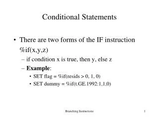
Conditional Statements • There are two forms of the IF instruction %if(x,y,z) • if condition x is true, then y, else z • Example: • SET flag = %if(resids > 0, 1, 0) • SET dummy = %if(t.GE.1992:1,1,0) Branching Instructions
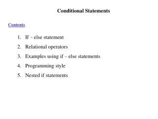
If-Else • IF condition 1 next statement or block executed if condition is true Examples 1. If x = = 0 display ‘Zero encountered’ 2. If x = = 0 { program statements } end if (needed when IF is not within a compiled section) • ELSE IFcondition n • ELSE • RATS performs the first IF or ELSE IF condition that is true. If all are false, RATS will perform ELSE (if present). Branching Instructions
Relational Operators • RATS uses the standard relational operators • A == B A.EQ.B • A <> B A.NE.B • A > B A.GE.B • A < B A.LT.B • A >= B A.GE.B • A <= B A.LE.B • A.AND.B • A.OR.B Branching Instructions
If-Else Examples Example 1 IF COUNT>=5 DISPLAY 'COUNT IS GREATER THAN OR EQUAL TO 5' ELSE DISPLAY 'COUNT IS LESS THAN 5' END IF Example 2 Examples of both types of IF are in PHI_NO.PRG Example 3: Bootknown.prg Branching Instructions
Notes Series vs. Constants • There is an important distinction between a series and a constant. A constant is a single number (i.e., a scalar). A series is a ‘vector’ of numbers. • compute a = 5 • compute a = 5.0 • set a = 5 • set a = 5.0 • The first crates an integer a, the second creates the floating point number 5.0, the third creates a series with each element equal to the integer 5, the last creates a series with each element equal to the floating point number 5.0. • You cannot switch a ‘character’ between a series and a constant. • You can use multiple assignments on a COM statement • e.g., com a = 5, b = 3.2, c = d = f = 4. • COM can perform all standard numerical operations Branching Instructions
Dates as Integers • If CAL is used, each date can be expressed as an integer or in RATS date form. • It is not necessary to use CAL. You can begin a program with: • ALLOCATE 100 Branching Instructions
DATES as Integers: Example cal 1947 1 4 all 2003:2 open data c:\\gdp.xls data(format=xls,org=obs) / There are 226 observations between 1947:1 and 2003:2. The following statements are equivalent to those above: all 226 open data c:\\gdp.xls data(format=xls,org=obs) / To estimate a regression over the first 100 observations use: LIN rcons 1 100 # constant trend t2 Branching Instructions
Series as Integers • Each series has its own sequence number. The number can be determined from the position of the series obtained from TABLE / • Example from gdp.xls table • Series Obs Mean Std Error Minimum Maximum • RGDP 214 4350.07009346 2128.96321099 1481.70000000 9311.50000000 • RCONS 214 2856.75700935 1461.19505124 963.40000000 6258.20000000 • RINV 214 616.25560748 383.72298968 153.90000000 1862.40000000 Here rcons is series 2 Branching Instructions
Series as Integers II • Anywhere RATS expects a series name, you can use the sequence number. • The series number is an integer • EXAMPLES using gdp.xls • print / 1 3 [prints rgdp and rinv] • print / 1 to 3 [prints rgdp, rcons and rinv] • lin 2 # constant 2{1} • To check the series number, you can also use: • com snum = rgdp ; dis snum Branching Instructions
Series as Integers III • Care must be taken if a series is on the right hand-side of a FRML, SET or COM instruction since RATS will interpret the integer as a scalar. On the right hand side use: [series]number • Example: You want to SET y equal to the log of series 2 • NOT: set y = log(2) • USE: set y = log([series]2) Branching Instructions
Rats Programming Language Loops • Do i = 1,100,increment program statements end do i Notes: The increment is optional BUT i must always take on integer values. The increment can be negative Loops can be nested BUT each must have its own end do. end do can be used instead of end do i Example: DO REGEND=1994:1,1994:12 LINREG Y 1980:1 REGEND # CONSTANT X1 X2 END DO Branching Instructions
Loops Loops • Do i = 1,100,increment program statements end do i Notes: The increment is optional BUT i must always take on integer values. The increment can be negative Loops can be nested Example: DO LAST = 1994:1,1994:12 LINREG Y 1980:1 LAST # CONSTANT X1 X2 END DO Branching Instructions
Loops II Example 2 do ar = 1,3 do ma = 1,3 box(constant,ar=ar,ma=ma) y end do ma end do ar 2. DOFOR index = list of values end dofor The index can be almost any type of variable Example dofor j = rgdp rcons lin j ; # constant j{1} end dofor Branching Instructions
3. WHILE condition { program statements } end while 4. UNTIL condition { program statements } end while 5. Branch label :label This is an unconditional jump 6. LOOP break end loop This will cycle forever until break is encountered Loops III Branching Instructions
Loops and Date Manipulation 1. DO REGEND=1994:1,1994:12 LINREG Y 1980:1 REGEND # CONSTANT X1 X2 END DO Is Equivalent to: 2. DO I =169,180 LINREG Y 1980:1 I # CONSTANT X1 X2 END DO I Branching Instructions
Loops and Series Manipulation Example 1: do i = 1,5 lin i # constant i{1} x end do i Example 2: Loops.prg: The program illustrates date and series manipulations using real exchange rate data. Branching Instructions
Introduction to Monte Carlo Analysis • The goal is to recreate a random outcome many times is order to assess the probability distribution of the outcome. • In RATS you can create random numbers using: • %ran(x) • %uniform(x1,x2) • Example: • SET x = %ran(1) • You can obtain the fractiles using: STATISTICS(FRACTILES) or FRACT.SRC • NOTE: The DENSITY Instruction will estimate an entire density function • EXAMPLE: MONTE.PRG Branching Instructions
Introduction to Bootstrapping • In bootstrapping, we typically perform a type of Monte Carlo analysis but we use a particular data set to generate the random variables. • Examples: • bootgdp.prg Branching Instructions
Simulating a Single Equation • SIMULATE 1 steps start # equation forecasts forstart Supplementary Information equation: the equation name or number forecasts: series for simulated values newstart: starting entry for storing values (default: start) Example: lin(define=eq1) y ; # constant y{1} SIMULATE 1 100 70:1 # eq1 fores Simulates a model with random Normally distributed shocks. An error in RATS 5.0 See Simulations.prg (USE RATSW) Branching Instructions
Simulating Multiple Equations • You can create a model using SYSTEM or GROUP. and them use SIMULATE. One way to use SIM is: SIMULATE(model=model,results=output) * steps start VCM model = model to simulate results = vector[series] for result series This provides a VECTOR of SERIES which will be filled with the results. For instance, RESULTS=SIMULS will make SIMULS(i) the series of simulations for the ith equation in the model. Branching Instructions
Example Using SIMULATE system(model=var1) 1 to 3 vars x1 x2 x3 lags 1 to 4 det constant end(system) estimate(noprint,noftests,outsigma=v) do i = 1,1000 SIMULATE(Model=var1,results=outpt) 3 24 %sigma program statements involving outpt end do i Branching Instructions

