Download
1 / 19
190 likes | 308 Vues
Simulations of Coastal Dispersal and Creek Runoff. Collaborators: Leonel Romero (UCSB) Jim McWilliams (UCLA) , Yusuke Uchiyama (Kobe University ), and Carter Ohlmann (UCSB). Work in Progress. Coastal dispersion nearshore

E N D
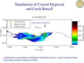
Simulations of Coastal Dispersal and Creek Runoff • Collaborators: Leonel Romero (UCSB) Jim McWilliams (UCLA) , Yusuke Uchiyama (Kobe University), and Carter Ohlmann (UCSB)
Work in Progress • Coastal dispersion nearshore -Characterization of lateral dispersal within 15 km from the coast in Southern California -Bays vs Headlands: coastal geometry, depth, current variability and a measure of the strain due to eddies. -Simple scalings and parameterization of the relative dispersion nearshore 2) Creek runoff simulation from Mission Creek and Arroyo Burro in the Santa Barbara Channel • Three significant storms in January 2008 • Characterization of the plume with different metrics • Temporal mean, distribution of maximum concentration, period exceeding a threshold (lethal dose) • Spatiotemporal evolution of freshwater plumes.
Regional Ocean Model System (ROMS) Nested Configuration Downscaling: 5km1 km 250 m 100 m* Buijsman et al. 2011
Surface Salinity and Vertical Vorticity Innermost solution (100 m – resolution) embedded in parent solution (250m ) + • Vertical Vorticity normalized by the Coriolisparameter • web link: http://youtu.be/Uo389p_g8aY
Coastal Discharge Model • Regional Ocean Model System (ROMS) -River runoff (boundaries) and effluent flow (bottom) • Input parameters: • Discharge , tracer concentration, temperature, and salinity. • Current work in SBC (Arroyo Burro and Mission Creek) • Inputs: LTER data discharge, temperature, salinity=0, tracer concentration at the source =1. • The discharge is distributed across three pixels (100x100m) and over 1.5 m of water (min depth)
Winter 2008/2008 Hydrographs at Arroyo Burro and Mission Creek
Hydrograph from Arroyo Burro (Jan. 2008) Net volume discharge from each storm at Arroyo Burro is about 6 x 10⁵ m3
River Runoff from Arroyo Burro and Mission Creek -Simulation of Vertically integrated tracer concentration (or freshwater fraction) Period shown: Dec 27, 2007 – Feb 20, 2008 http://youtu.be/LHyd9_Y_OPs Mohawk Reef Arroyo Burro Mission Creek
River Runoff from Arroyo Burro and Mission Creek Simulation of Vertically integrated tracer concentration (or freshwater fraction) Period shown: Dec 27, 2007 – Feb 20, 2008 http://youtu.be/99um5DNbQw8
Mean and Maximum Freshwater Fraction per Storm Arroyo Burro discharge Mission Creek discharge Averaging Interval Mohawk Reef Arroyo Burro Mission Creek
Duration of Tracer Exceeding 1% Arroyo Burro discharge Mission Creek discharge Time Interval Mohawk Reef Arroyo Burro Mission Creek
Spatiotemporal Distributions Arroyo Burro Mean distributions calculated over 5 km from the coast and within 30 km from the creek along-shelf. 1st storm in January 2008.
Spatial Anisotropy Cross-shelf Along- shelf *Degree of anisotropy ~ 10 (c.f. Romero et al. 2013) Storms in January 1st 2nd 3rd
Future and Ongoing Work • Increase the number of storms: 2004/2005 • (Collaboration with Charles Jones, UCSB – meteorological forcing) • Analysis of the flow fields including statistics, and vertical structure of the plumes. • Characterization of dilution field: distance and direction from the source, current variability, straining by eddies, and wind stress. • Quantification of the along- and cross-shelf diffusivity based on the spatiotemporal evolution of the dilution field (diffusion model) • Quantification of the diffusivity based on moments of the dilution fields. • Simple model describing the dilution field with parametric dependent on respect to the discharge rate, wind stress, current variability, and straining by eddies.
3D Plume Structure ocean surface (a) Vertical Cross Sections (b) (e) (c) (f) (d) (g)
Eddy Kinetic Energy • Headlands have more energy than Bays by up to a factor of 10.
Particle Release Strategy and Regions “Bays” “Headlands” • About 1000 particles are released near the surface (10m depth) every half a day and are tracked for about 5 days. • Two release sites per geographic region • Releases are repeated continuously for one season (4 months) • Two-particle statistics within each of the predetermined regions