
Solving the Optimal Trading Trajectory Problem Using a Quantum Annealer
E N D
Presentation Transcript
Solving the Optimal Trading Trajectory Problem Using a Quantum AnnealerGili Rosenberg, PoyaHaghnegahdar, Phil Goddard, Peter Carr, Kesheng Wu, and Marcos Lopez de Prado
Objective • Give a brief introduction to the portfolio optimization problem • Give a brief introduction to quantum annealing • Illustrate how the portfolio optimization problem can be solved on the D-Wave's quantum annealer • Look at the experimental results • Describe the problems faced and the limitations of the work • Think about whether it makes sense to actually execute real life problems on the D-Wave, based on the experimental results obtained
Portfolio Optimization • Process of selecting the best portfolio out of multiple portfolios, according to some objective • Objective typically involves maximizing expected return and minimizing risk • Constrained utility-maximization problem • NP-complete problem • Central to the solution of this problem is the construction of a covariance matrix
Crux of the Problem • Asset manager wants to invest K dollars in a set of N assets with an investment horizon divided into T time steps • Asset manager has to decide how much to invest in each asset at each time step • Has to take into account transaction costs, and the behavior of the market
Solution • Compute the portfolio that maximizes the return subject to a level of risk at each time step • Results in a series of statically optimal portfolios • Cost of rebalancing from a portfolio that is locally optimal at t to a portfolio that is locally optimal at t+1 • Might result in the formulation of a less optimal portfolio than the globally optimal portfolio • Traditionally solved as continuous-variable problems • However for large assets, a discrete solution yields better results
Integer Formulation The first term is the sum of the returns at each time step, which is given by the forecast returns μ times the holdings w. The second term is the risk, in which the forecast covariance tensor is given by Σ, and γ is the risk aversion. The third and fourth terms encapsulate transaction costs
What is Quantum Annealing • Way of using the intrinsic effects of quantum physics to solve • Optimization Problems • Find best configuration amongst many possible configurations • Can be represented as an energy minimization problem • Probabilistic Sampling • Related to optimization problems • Instead of finding minimum energy state, sample many low energy states to characterize the shape of energy landscape
Use of Quantum Annealers Quantum Annealers • are designed to solve certain problems • using a quantum annealing algorithm • that belongs to the adiabatic quantum model of computation • and is implemented in hardware that exploits quantum properties
Adiabatic Quantum Optimization Perspective Slide taken from Joel Gottlieb's talk: Introduction to the Physics of D-Wave and Comparison to the Gate Mode
Adiabatic Quantum Computation Steps for adiabatic quantum computation • First, a Hamiltonian is found whose ground state describes the solution to the problem of interest • Then, a system with a simple Hamiltonian is prepared and initialized to the ground state • Finally the simple Hamiltonian is adiabatically evolved to the desired complicated Hamiltonian
D-Wave Quantum Annealer • Device which minimizes unconstrained binary quadratic functions • Cooled to 15 mK to keep disturbances at a minimum • Shielded from RF signals • Shielded from external magnetic fields larger than 1 nT • Operates in a high vacuum environment
D-Wave application flow • Recast variables in original problem as binary variables • Convert to Quadratic Unconstrained Binary Optimization (QUBO) • Solve QUBO with qbsolv • Convert bit vector back to variables in problem domain • Interpret qbsolv results and adjust accordingly Steps taken from Joel Gottlieb's talk: Driving to the 48 USA State Capitals: Programming the D-Wave QPU
Chimera Graph(contd.) • Describes the connectivity of D-Wave's quantum annealer • Sparsely connected graph with a well-defined structure of edges • For square Chimera hardware graphs, the size V of the largest fully dense problem that can be embedded on a chip with q qubits is V = √2q +1=4s + 1, where s is the number of unit cells along an edge • To solve problems that are denser than the hardware graph, multiple physical qubits are identified with a single logical qubit, at the cost of using many more physical qubits
From Integer to Binary • To solve the optimization problem on the Quantum annealer, the variables in the equation given on slide 8 have to be recast as binary variables • Four different encodings investigated for the purpose: • Binary - representation of symbols in a source alphabet by strings of binary digits • Unary - representation a natural number, n, with n ones followed by a zero • Sequential - approximate decoding algorithm for long constraint-length convolutional codes • Partitioning – find all partitions of K into N assets, and assign a binary variable to each encoding at each time step
Binary Encoding • Number of variables required to represent a particular problem is T*N*log2(K' + 1) • Largest integer that can be represented is [2n] - 1 • Most efficient in number of variables • Allows representation of the second-lowest integer • Requires the least number of variables • Most sensitive to noise
Unary Encoding • Number of variables required to represent a particular problem is T*N*K' • No limit on the largest integer that can be represented • Biases the quantum annealer due to differing redundancy of code words for each value • Encoding coefficients are even, giving no dependence on noise, so it allows representing of the largest integer • Requires the second largest number of variables
Sequential Encoding • Number of variables required to represent a particular problem is ½*T*N*(√(1+8K') − 1) • Largest integer that can be represented is ½*[n]*([n] + 1) • Biases the quantum annealer (but less than unary encoding) • Second-most-efficient in number of variables • Allows representing of the second-largest integer
Partition Encoding • Number of variables required to represent a particular problem is less than or equal to T*(K+N-1) or T*(N-1) • Largest integer that can be represented is [n] • Can incorporate complicated constraints easily • Least efficient in number of variables • Only applicable for problems in which groups of variables are required to sum to a constant • Allows representing the lowest integer.
Number of BinaryVariables Used As we can see, unary encoding requires the maximum number of variables, compared to the other two encodings
Results Success rate increases while using 1Qbit's solver
Results(contd.) The 1152-Qubit Quantum Annealer has a higher success rate than the 512-Qubit Quantum Annealer
Success Rate • As a solution metric, the percentage of instances for each problem for which the quantum annealer’s result fell within perturbation magnitude α% of the optimal solution were used • The metric was evaluated by perturbing each instance at least 100 times, by adding Gaussian noise with standard deviation given by α% of each eigenvalue of the problem matrix Q • Each perturbed problem was solved by an exhaustive solver, and the optimal solutions were collected • If the quantum annealer’s result for that instance fell within the range of optimal values collected, then it was deemed successful
Problems • Level of intrinsic noise which manifests as a misspecification error • Coefficients of the problem that the quantum annealer actually solves differ from the problem coefficients by up to Ɛ. Problem coefficients on the chip have a defined coefficient range, and if the specified problem has coefficients outside this range, the entire problem is scaled down, resulting in coefficients becoming smaller than Ɛ, affecting the success rate
Problems(contd.) • To solve problems that are denser than the hardware graph, multiple physical qubits are identified with a single binary variable, at the cost of using more physical qubits • To force the identified qubits to all have the same value, a strong coupling is needed • More qubits needed, as more qubits would allow the use of an encoding scheme that is less sensitive to noise levels • Better error correction required
Speedup • There is an ongoing debate on how to define quantum speedup • For the small-scale problems solved in this study, the time to solution, on both classical hardware and using the quantum annealer, is COMPARABLE • Only after quantum speedup has been demonstrated for general problems, and specifically those requiring a high precision of couplings, is it expected that a quantum speedup for the optimal trading trajectory problem will be observed
Conclusion • Demonstrated the potential of D-Wave’s quantum annealer to achieve high success rates while solving the portfolio optimization problem • Possible to achieve a considerable improvement in success rates by finetuning the operation of the quantum annealer • Technological improvements in future generations of quantum annealers are expected to provide the ability to solve larger problems, and at higher success rates