Modeling Negative Power Law Noise
200 likes | 339 Vues
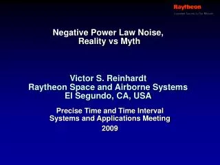
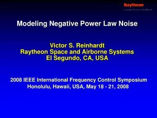
Modeling Negative Power Law Noise . Victor S. Reinhardt Raytheon Space and Airborne Systems El Segundo, CA, USA. 2008 IEEE International Frequency Control Symposium Honolulu, Hawaii, USA, May 18 - 21, 2008. f -1. dBc/Hz. f -2. f -4. f -3. Log 10 (f).

Modeling Negative Power Law Noise
E N D
Presentation Transcript
Modeling Negative Power Law Noise Victor S. ReinhardtRaytheon Space and Airborne SystemsEl Segundo, CA, USA 2008 IEEE International Frequency Control Symposium Honolulu, Hawaii, USA, May 18 - 21, 2008
f -1 dBc/Hz f -2 f -4 f -3 Log10(f) Negative Power Law Noise Gets its Name from its Neg-p PSD • But autocorrelation function must be wide-sense stationary (WSS) to have a PSD • Then can define PSD LX(f) as Fourier Transform (FT)over of Rx() tg = Global (average) time = Local (delta) time
Neg-p Noise Also Called Non-Stationary (NS) • Must use dual-freq Loève spectrum Lx(fg,f) not single-freq PSD Lx(f) • Loève Spectrum • Paper will show neg-p noise can be pictured as either WSS or NS process • And these pictures are not in conflict • Because different assumptions used for each • Will also show how to generate practical freq & time domain models for neg-p noise • And avoid pitfalls associated with divergences
Random Walk v-2(t) t White Noise Vo 1/j - V-2 1 Classic Example of Neg-p Noise – Random Walk • Integral of a white noiseprocess is a random walk • But starting in f-domain • Can write • So • Because • Will show different assumptions used for each picture so not in conflict Not WSS f-domain Integrator Is WSS?
Random Walk 2(tg)tg A Historical Aside — Random Walk • 1st discussed by Lucretius [~ 60 BC] • Later Jan Ingenhousz [1785] • Traditionally attributed toRobert Brown [1827] • Treated by Lord Rayleigh [1877] • Full mathematical treatment by Thorvald Thiele [1880] • Made famous in physics by Albert Einstein [1905] and Marian Smoluchowski [1906] • Continuous form named Wiener process in honor of Norbert Wiener
Lo H(f) |H(f)|2Lo(f) Generating Colored Noise from White Noise Using Wiener Filter • Can change spectrum of white noise v0(t) by filtering it with h(t),H(f) • H(f) called a Wiener filter • NS picture • Starts at t=0 • WSS picture • Must start at t=- for t-translation invariance • Necessary condition for WSS process • Wiener filters divergent for neg-p noise • Need to write neg-p filter aslimit of bounded sister filterto stay out of trouble Wiener Filter
0 he(t-t’) 1/ t t’ 1/j - V V0 0 1 Sister Filter -1 |He(f)|-dB Log(f) Random Walk as the Limit of a Sister Process • Sister process is single poleLP filtered white noise • In WSS picture v-2(t) = for any t • Need sister processes to keep v-2(t) finite • True for any neg-p value
WSS PictureofRandom Walk v-2(t) - NS Picture ofRandom Walk v-2(t) 0 t Even When Final Variable Bounded (Due to HP Filtering of Neg-p Noise) • Intermediate variables areunbounded (in WSS picture) • Can cause subtle problems • Sister process helps diagnose& fix such problems • In NS picture v-2(t) isbounded for finite t • But v-1(t) (f -1 noise) is not • Sister process needed forf -1 noise even in NS pictureto keep t-domain process bounded
Models For f -1 Noise • The diffusive line model • White current noise into a diffusive line generates flicker voltage noise • Diffusive line modeled as R-C ladder network • In limit of generates f -1 voltage noise with white current noise input
Sister Model for Diffusive Line • Adds shunt resistor to bound DC voltage • Not well-suited for t-domain modeling • Because Wiener filter not rational polynomial
A Historical Aside — The Diffusive Line • Studied by Lord Kelvin [1855] • For pulse broadening problem in submarine telegraph cables • Refined by Oliver Heaviside [1885] • Developed modern telegrapher’s equation • Added inductances & patented impedance matched transmission line • Adolf Fick developed Fick’s Law & diffusion equation [1855] • 1-dimensional diffusion equation following Fick’s (Ohm’s) Law is diffusive line • Used in heat & molecular transport
0 0 V0,0 V-1 ●● ●● V0,m M V0,M The Trap f -1 Model is More Suited for f & t Domain Modeling • Each “trap” independentwhite noise source filteredby single-poleWiener filter • Sum over m from 0 to M • Sister model (M )0> 0 M< • Well-behaved inf & t domains • For 0 0 M becomes f -1 noise (L0 same for all m)
A Historical Aside — The Trap Model • Developed by McWorter [1955] to explain flicker noise in semiconductors • Traps loosely coupled storage cells for electrons/holes that decay with TCs 1/m • Surface cells for Si & bulk for GaAs/HEMT • GaAs/HEMT semi-insulating (why much higher flicker noise) • Simplified theory by van der Ziel [1959] • Flicker of v-noise from traps converted to flicker of -noise in amps through AM/PM
0 L-1(f) -20 dB L(f) -40 -60 0 2 4 6 Log(f) Error from f -1 = ±1/4 dB +1/4 dB -1/4 A Practical Trap Simulation Model Using Discrete Number of Filters • Trap filter every decade • ±1/4 dB error over 6 decades with 8 filters • Can reduce error by narrowing filter spacing
Other f -1 Noise Models • Barnes & Jarvis [1967, 1970] • Diffusion-like sister model with finite asymmetrical ladder network • Finite rational polynomial with one input white noise source • 4 filter stages generate f -1 spectrum over nearly 4 decades of f with < ±1/2 dB error • Barnes & Allan [1971] • f -1 model using fractional integration
Discrete t-Domain Simulators for Neg-p Noise • For f -2 noise can use NS integrator model in discrete t-domain • NS model bounded in t-domain for finite t • Discrete integrator (1st order autoregressive (AR) process) • wn = uncorrelated random “shocks” or “innovations” • wn need not be Gaussian (i.e. random ±1) to generate appropriate spectral behavior • Central limit theorem Output becomes Gaussian for large number of shocks
Spectrum Recovered from t-Domain Simulation FittedSlope f -1.03 Log10(L(f)) from xn Log10(f) Trap f -1 Discrete t-Domain Simulator • Must use sister model • Full f -1 model unboundedin NS picture • Wiener filter for each trap • t-domain AR model • Sum overtraps forf -1 noise
WhiteInput f 0 WhiteInputs Trapf -1 f -1 WhiteInput Integratef -2 f -2 WhiteInputs Trapf -1 Integratef -2 f -3 WhiteInput Integratef -2 Integratef -2 f -4 From f -1 and f -2 models Can Generate any Integer Neg-p Model Right Crop 66%x72%
Summary and Conclusions • Either WSS or NS pictures can be used for neg-p noise as convenient • Not in conflict Different assumptions used • Need sister models to resolve problems • Can generate practical models for any integer neg-p noise • By concatenating integrator & trap models • Are simple to implement in f & t domains • For preprint & presentation see www.ttcla.org/vsreinhardt/