Chapter 9: Boundary Testing
Chapter 9: Boundary Testing. Input Domain Partitioning Simple Domain Analysis and Testing Important Boundary Testing Strategies Extensions and Perspectives. Non-Uniform Partition Testing.

Chapter 9: Boundary Testing
E N D
Presentation Transcript
Chapter 9: Boundary Testing • Input Domain Partitioning • Simple Domain Analysis and Testing • Important Boundary Testing Strategies • Extensions and Perspectives
Non-Uniform Partition Testing • Extensions to basic partition testing ideas include Non-uniform or Selective or partitioned testing strategies • Testing is based on related problems: some sub-domains will be tested more • Usage-related problems => Use Musa’s Ops and UBST • Sub-domains with complex boundary problems => Use input domain boundary testing (BT).
Boundary Testing: Overview • What is it? • Test I/O relations. • Classifying/partitioning of input space • Cover input space and related boundary conditions. • Also called (input) domain testing. • Characteristics and applications? • Functional/black-box view (I/O mapping for multiple sub-domains) • Well-defined input data: • numerical processing and decisions. • Implementation information may be used => then more white box • Focus: boundaries and related problems. • Output used only in result checking.
I/O Variables and Values • Input: • Input variables: x1, x2,. . . , xn. • Input space: n-dimensional. • Input vector: X = [x1, x2, . . . , xn]. • Test point: X with specific xi values. • Domains and sub-domains: specific types of processing are defined. • Focus on input domain partitions. • Output (assumed, not the focus) • Output variables/vectors/space/range similarly defined. • Mapped from input by a function. • Output only used as oracle.
Domain Partitioning and Sub-domains • Input domain partitioning • Divide into sets of sub-domains. • “domain", “sub-domain", and “region“ often used interchangeably • A sub-domain is typically defined by a set of conditions in the form of: f(x1, x2, ..., xn) < K where “<" can also be substituted by “>", “=", “≠", “<", or “>".
Domain Partitioning and Sub-domains • Domain (sub-domain) boundaries: • Distinguishes/defines different sub-domains. • Each defined by it boundary condition, e.g., f(x1, x2, ., xn) = K • Adjacent domains: those share common boundary(ies) • Boundary properties and related points: • Linear boundary: a1x1 + a2 x2, ., +anxn = K (Otherwise, it is a nonlinear boundary.) • Boundary point: point on the boundary. • Vertex point: 2+ boundaries intersect. • Other properties w.r.t domains later.
Boundary and Domain Properties • Boundary properties w.r.t domains: • Closed boundary: inclusive (<, > ) • Open boundary: exclusive (<, >) • Domain properties and related points: • Closed domain: all boundaries closed • Open domain: all boundaries open • Linear/nonlinear domain: all linear boundary conditions? • Interior point: in domain and not on boundary. • Exterior point: not in domain and not on boundary.
Input Domain Partition Testing • General steps: • Identify input variable/vector/domain. • Partition the input domain into sub-domains. • Perform domain/sub-domain analysis. • Define test points based on the analysis. • Perform test and follow-up activities. • Boundary testing: Above with focus on boundaries. • Domain analysis: • Domain limits in each dimension. • Domain boundaries (more meaningful). • Closure consistency? • Plotting for 1D/2D, algebraic for 3D+.
Problems in Partitioning • Domain partitioning problems: • Ambiguity: under-defined/incomplete. • Contradictions: over-defined/overlap. • Most likely to happen at boundaries. • Related boundary problems: • Closure problem. • Boundary shift: f(x1, x2, ., xn) = K+δ • Boundary tilt: parameter change(s). • Missing boundary. • Extra boundary.
Simple Domain Analysis and EPC • Simple domain analysis: identify domain limits in each dimension. • Extreme point combinations (EPC) • Combine with above to derive test points. • Each variable: under, min, max, over. • Combine variables (× cross-product). • Examples: Fig 9.1&9.2 (p.133-134)
Simple Domain Analysis and EPC • Problems/shortcomings with EPC: • Missing boundary points: 2D example, unless boundaries perfectly aligned. • Exponential # test cases: 4n +1. • Vertex points appropriate? => Need more effective strategies.
Boundary Testing Ideas • Using points to detect boundary problems: • A set of points selected on or near a boundary: ON and OFF points. • Able to detect boundary movement, tilt, etc. • Motivational examples for boundary shift. • Є neighborhood and ON/OFF points • Region of radius around a point • Є = 1/2n for n binary digits after decimal • ON point: On the boundary • OFF point: • opposite to ON processing • off boundary, within distance • closed boundary, outside
Weak N × 1 Strategy • N x 1 strategy • N ON points (linearly independent. • 1 OFF point: centroid of ON points. • Weak: set of tests per boundary instead of per boundary segment. • # test points: (n+1) × b+1 • Examples: Fig 9.3 & 9.4 (p.137/138). • Advantages (esp. 2D) over EPC!
Weak N × 1 Strategy • Typical errors detected: • Closure bug • Boundary shift • Boundary tilt: Fig 9.5 (p.138) • Extra boundary (sometimes) • Missing boundary
Weak 1 × 1 • Motivation: # test-points goes down without losing much of the problem detection capability. • Characteristics: • 1 ON and 1 OFF per condition (sample of n ON points in weak N × 1 form an equivalent class) • Key: boundary defined by ON/OFF • Typical errors detected: • Closure bug • Boundary shift • Boundary tilt (sometimes!) (Fig 9.7 vs Weak N × 1) • Missing boundary • Extra boundary (sometimes)
Other BT Strategies • Strong vs weak testing strategies: • Weak: 1 set of tests for each boundary • Strong: 1 set of tests for each segment • Why use strong BT strategies? • Gap in boundary condition • Closure change • Coincidental correctness: particularly stepwise implementation • Code clues: complex, convoluted • Use in safety-critical applications • Nonlinear boundaries: Approximate (e.g., piecewise) strategies often useful.
BT Extensions • Direct extensions • Data structure boundaries, e.g. arrays. • Capacity testing. • Loop boundaries (Ch.11). • Other extensions • Vertex testing: • problem with boundary combinations • follow after boundary test (1X1 etc.) • test effective concerns • Output domain in special cases • similar to backward chaining • safety analysis, etc. • Queuing testing example below.
Queuing testing as Boundary Testing • Queuing description: priority, buffer, etc. • Priority: time vs other: • time: FIFO/FCFS, LIFO/stack, etc. • other/explicit: SJF, priority#, etc. • purely random: rare • Buffer: bounded or unbounded? • Other information: • Pre-emption allowed? • Mixture/combination of queues • Batch and synchronization • Example: prioritized, w/o pre-emption or batching
Testing a Single Queue • Test case design/selection: • Conformance to queuing priority. • Boundary test • Test cases: input + expected output. • Combined cases of the above. • Testing specific boundary conditions: • lower bound: 0(empty), 1, 2 (test insertions) • server busy/idle at lower bound – is arrival served immediately? • upper bounds: B-1 (new arrival pushed Q to capacity), B (full), and B + 1 (similar to OFF point) • Other test cases: • Typical case: usage-based testing idea. • Q unbounded: some capacity testing.
BT Limitations • Simple processing/defect models: • Processing: case-like, general enough? • Specification could be ambiguous/contradictory. • Boundary: likely defect. • Vertex: ad hoc logic. • Limitations • Processing model: no loops. • Coincidental correctness: common. • Є-limits, particularly problematic for multi-platform products. • OFF point selection for closed domain • possible undefined territory, • may cause crash or similar problems. • Detailed analysis required.