Download

1 / 20
200 likes | 341 Vues
Fitting Cox regression models ALDA, Chapters Fourteen and Fifteen. “Time is nature’s way of keeping everything from happening at once” Woody Allen. Judith D. Singer & John B. Willett Harvard Graduate School of Education. Chapters 14 & 15: Fitting Cox regression models.

E N D
Fitting Cox regression modelsALDA, Chapters Fourteen and Fifteen “Time is nature’s way of keeping everything from happening at once” Woody Allen Judith D. Singer & John B. Willett Harvard Graduate School of Education
Chapters 14 & 15: Fitting Cox regression models • Towards a statistical model for continuous-time hazard (§14.1)—how it is similar to, and different from, the discrete-time hazard model • Biggest difference—you don’t actually estimate the baseline hazard function! • Fitting the the continuous time hazard model to data (§14.2)—Cox regression—also known as the proportional hazards model—is very straightforward to implement and interpret • Evaluating the results of model fitting (§14.3)—interpreting parameter estimates, testing hypotheses, evaluating goodness of fit, and summarizing effects • Graphically displaying the results of model fitting (§14.4)— • A tad more difficult because you don’t actually estimate the baseline hazard function • Including time-varying predictors (§15.1)—It’s not always as easy as in discrete-time, but it can be done • Non-proportional hazards models (§15.2)—One of the major advantages of learning how to include time-varying predictors is that they allow you to test and, if necessary, relax the proportional hazards assumption
Example for fitting Cox regression models Person-level data set (note, we do not use a person-period data set) • AGE at release—centered on sample mean of 30.7 • PERSONAL—identifies the 61 former inmates (31.4%) who had a history of person-related crimes (e.g., assault, kidnapping) Event occurrence information • PROPERTY—identifies the 158 (81.4%) who had a history of property crimes Data source: Kristin Henning and colleagues, Criminal Justice and Behavior • Sample:194 inmates released from a minimum security prison • Research design • Each was followed for up to 3 years • Event: Whether and, if so, when they were re-arrested • Arrest recorded to the nearest day • N=106 (54.6%) were reincarcerated
Towards a statistical model for continuous-time hazard:Sample functions by levels of PERSONAL Survivor functions: Recidivism is high in both groups,although those with a history of person-related crimes are clearly at greater risk (ML of 17.3 vs. 13.1) • Intuitively, a continuous-time hazard model should look like a DT hazard model, where some transformation of hazard is expressed as the sum of two components: • A baseline function, the value of transformed hazard when all predictors are 0 • A weighted linear combination of predictors • Realistically, because we lack a complete picture of hazard, we instead develop the model in terms of cumulative hazard. After doing so, we use transformation to specify an equivalent model in terms of hazard. Cumulative hazard functions: Approximately linear immediately after release and soon accelerates (but at slightly different times); eventually both decelerate. Suggests that each underlying hazard function is initially steady, then rises, then falls. Kernel-smoothed hazard functions: Can’t describe risk immediately after release, but by month 8, we can see that the hazard for PERSONAL=1 is consistently higher than the hazard for PERSONAL=0 (ALDA, Section 14.1.1, pp. 504-507)
Towards a statistical model for cumulative hazard Log H(t ) A baseline function, now the value of log H(t) when all predictors are 0 j 1.00 A weighted linear combination of predictors 0.00 PERSONAL = 1 -1.00 Solution: model log cumulative hazard (which is defined for any positive value) -2.00 PERSONAL = 0 -3.00 compresses the distance between larger values -4.00 -5.00 expands the distance between small values -6.00 0 6 12 18 24 30 36 But, how do we specify this baseline? As in DT, we use a completely general unconstrained shape, which we’ll call log H0(tj) Might think this vagueness creates problems for estimation, but the beauty of Cox’s approach is that it’s perfectly fine Months after release Problem: cumulative hazard is bounded, but only from below (by 0), so we can’t take logits What kind of statistical model should we use to model log H(t)? A dual partition still makes sense, where log H(t) is expressed as the sum of two parts: (ALDA, Section 14.1.1, pp. 504-507)
Specifying the Cox regression model in terms of log cumulative hazard When PERSONAL=1, the Baseline Function shifts “vertically” by 1 Mapping the model onto sample log cumulative hazard functions (using +’s and ’s to denote estimated subsample values) Log H(t ) ij 1.00 PERSONAL = 1 Vertical distance between functions, b1,assesses the magnitude of the predictor’s effect. (We assume that the effect is constant regardless of how long the offender has been out of prison) " " " " " " ! ! " ! 0.00 ! " ! ! " ! ! " ! Curves are hypothesized population log cumulative hazard functions (they should go through sample data but we don’t expect them to fit perfectly) ! " ! " ! " ! ! " ! ! " ! ! " ! " ! ! " ! ! " ! ! " ! ! " ! " ! ! ! " -1.00 ! ! " ! ! " ! " ! ! " ! ! " ! ! ! ! " ! PERSONAL = 0 ! " ! ! " ! ! -2.00 " ! ! b " ! Log H (t ) + ! ! " 0 j 1 ! ! " ! ! " ! -3.00 ! " ! ! -4.00 " ! ! Log H (t ) -5.00 0 j 0 6 12 18 24 30 36 Months after release (ALDA, Section 14.1.2, pp. 507-512)
Taking antilogs to specify the Cox regression model in terms of cumulative hazard When PERSONAL=1, the Baseline Function is no longer shifted vertically; instead, it is multiplied by exp(1) Mapping the model onto sample cumulative hazard functions (using +’s and ’s to denote estimated subsample values) Ratio of cumulative hazard functions Curves are hypothesized population cumulative hazard functions ratio=exp(b1) b H (t )exp( ) 0 j 1 H (t ) 0 j When the outcome is raw cumulative hazard, the functions are magnifications and dimunitions of each other—they are proportional Yet we still say the effect is constant over time because their ratio is constant (ALDA, Section 14.1.2, pp. 507-512)
Hazard function representation of the Cox regression model Through calculus, we can show that the Cox models just developed in terms of cumulative hazard are identical to those expressed in terms of raw hazard Raw hazard form Cumulative hazard form When expressed on a log scale, b1 represents a constant vertical distance When expressed on a raw scale, exp(b1) represents a constant vertical ratio • Practical consequences of this equivalence • We can do exploratory data analysis using cumulative hazard • We can interpret parameter estimates in terms of predictors’ effects on hazard • Because effects are proportional for raw hazard, the Cox model is often called a proportional hazards model (ALDA, Section 14.1.3, pp. 512-516)
Fitting the Cox regression model to data • 3 important practical consequences of Cox’s method: • The shape of the baseline hazard function is irrelevant. Unlike parametric methods—and there are many—we need not make any assumptions about the shape of the baseline hazard function—therefore, no assumptions about event time distributions are violated. • The precise event times are irrelevant; only their rank order matters. Cox regression is semi-parametric. The very data you took pains to collect precisely is effectively converted into ranks! • Ties can create analytic difficulties. Even though the specific values are irrelevant their ranking does matter. In theory, there should be no ties; in reality, there always are. (In the recidivism data, there are 5 days when 2 people were arrested—9, 77, 178, 207, & 528.) All packages have one or more approximations (we use Efron’s method). Estimation: In addition to specifying a particular model for hazard, Cox developed an ingenious method for model fitting data: partial maximum likelihood estimation (available in all major stat packages (See § 14.2)). (ALDA, Section 14.2, pp 516-523)
Interpreting parameter estimates in a fitted Cox regression model Overall model Simple uncontrolled models What does this look like graphically? Returning to the sample log cumulative hazard functions by PERSONAL, we estimate that in the population, the average distance between them is 0.479 Log hazard function for someone with a history of personal offenses is 0.479 units higher than for someone without this history Strategy for interpreting parameter estimates: Each assesses the effect of a 1-unit difference in the associated predictor on log hazard (controlling for all other predictors in the model) Is there a more intuitive way of explaining this? (ALDA, Section 14.3.1, p. 524-528)
Interpreting hazard ratios in a fitted Cox regression model Antilogged parameter estimates are fitted hazard ratios associated with a 1-unit difference in the predictor For continuous predictors Compute the %age difference in hazard associated with a 1-unit difference in the predictor: 100*(hazard ratio-1) e1.1946 100*(0.9342-1) = -6.58% The estimated hazard of recidivism is 6.6% lower for each additional year of age upon release The estimated hazard of recidivism among offenders with a history of property offenses is three times that of those with no such history Careful:Only make comparative statements about hazard You can say that the hazard for one group is three times higher than that of another, but you cannot say how high, or low, either function is This is the compromise associated with Cox regression (ALDA, Section 14.3.1, p. 524-528)
Summarizing findings using risk scores:Summarizing the effects of several predictors simultaneously A: By taking ratios of their hazard functions: risk score • At average comparative risk, but got there in different ways • ID 22 was average age with no history of these crimes • ID 8 had a history of both crimes but was 22 years older than the average inmate upon release • At low comparative risk • All are much older than average on release • None has history of both crimes • At high comparative risk • All are younger than average on release • ID 5 is over 7 times more likely than a baseline person to re-offend Q: How might you compare each person’s risk to that of the “baseline individual” (the person who really has all predictors = 0—here, someone of average AGE on release (30.7) who has no history of either PERSONAL or PROPERTY crime) Risk scores are useful for demonstrating that there is more than one way to attain a given level of risk but…. Careful: Changing the baseline by centering predictors changes risk scores (ALDA, Section 14.3.4, p. 532-535)
Recovered survivor and cumulative hazard functions Even though we have repeatedly stated that Cox regression provides no information about the baseline hazard function, it is possible to recover baseline functions from a model fit with time-invariant predictors (however, these are not predicted values) Useful for documenting the combined effects of predictors. Here, we use Model D to control for AGE and show the combined effect of PERSONAL and PROPERTY, documenting the large differences in survival associated with variation in these predictors (see Section 14.4 for details) (ALDA, Section 14.4, p. 535-542)
Including time-varying predictors in a Cox regression model Model specification is easy: Just add the subscript j to the time-varying predictors • Data demands can be high • (sometimes insurmountable) • You need to know the value of the time-varying predictor—for everyone still at risk—at every moment when someone experiences the event • Requirement holds whether there are 10, 100 or 1,000 unique event times • Same requirement as in discrete-time, but it was unproblematic there because: • Number of unique event times was relatively small • Event occurrence and predictors are typically assessed on the same schedule • In continuous time, you typically can’t set the data collection schedule to coincide with event occurrence for everyone still at risk • Practical implications • If you’re interested in TV predictors, research design is crucial—Don’t wait until the data are collected • Non-reversible dichotomies—that themselves represent event occurrence—are easiest (eg, 1st marriage, HS graduation) • Reversible dichotomies and continuous predictors usually require imputation(discussed in Section 15.1.2 and 15.1.3) (ALDA, Section 15.1, pp 544-545)
Including TV non-reversible dichotomies in a Cox regression model: Data example • Three time-invariant predictors • EARLYMJ and EARLYOD indicate whether the respondent had initiated marijuana (7.2%) or other drugs (3.7%) so early that he could be characterized as a previous user at t0(age 17) • BIRTHYR (1961-1985), to account for societal changes (included as a control predictor in every model) • Four time-varying predictors • USEDMJj, SOLDMJj USEDODj , SOLDODjeach identify, at each age tj , whether the respondent had previously used or sold marijuana (MJ) or other drugs (OD) • Conceptually, think about a person-period data set in which these variables switch from 0 to 1 in the relevant year and stay at 1 thereafter. • In reality, we do not use a person-period data set but rather computer code in a person-level data set ( Section 15.1, p. 547) • Rather than using contemporaneous values of the TV predictors, we lag them by one year.Addresses issues of rate-and state-dependence (discussed in Section 12.3.3, p. 440) Data source: Burton and colleagues (1996), Journal of Health and Social Behavior Sample:1,658 meninterviewed twice (in 1974 and 1985) -- 382 (23.0%) started using cocaine between ages 17 and 41 (ALDA, Section 15.1.1, pp 545-551)
Interpreting the results of fitting Cox regression models with time-varying predictors • Note: Diminishing BIRTHYR effects • Uncontrolled estimate=0.2026 • Drops from .1551 to 0.0849 from A to C • Effects previously attributable to BIRTHYR get absorbed by TV drug use (known as substitution effects) • C: Add • TV sales predictors • Creates ordinal variable when paired with use predictors • Both use and sales are stat sig. • Hazards add up: Someone who both used and sold MJ and OD has a hazard ratio of exp(5.1606)=164.27! • Best fitting model so far A: Only time-invariant predictors: All 3 stat sig • D: Add back time-invariant predictors • Estimates are not stat sig. • D fits no better than C • We prefer model C • B: Substitute • TV use predictors • Effects much larger (and still stat sig.) • Fit much better (use AIC because non-nested) (ALDA, Section 15.1.1, pp 545-551)
Might the effect of a predictor vary over TIME? Does this non-significant effect mean that the TREATment has no effect? Perhaps, but not necessarily…It could be that the effect of TREATment varies over time Fitted Cox model for TREAT Data source: Michael Foster and colleagues (1996), Evaluation and Program Planning • Sample:174 teens admitted to a psychiatric hospital • Research Design: True experiment • Half (n=88) had traditional psychiatric treatment and services (TREAT=0) • The other half (n=86) were randomly selected to participate in an innovative program that provided coordinated mental health services regardless of setting (in- or out-patient) • Everyone tracked for up to 3 months to determine whether and, if so, when they were released • RQ: Does provision of comprehensive mental health services reduce the length of hospital stay? (ALDA, Section 15.3.2, pp 564-570)
How might we detect a violation of the proportional hazards assumption? TREATment effect appears large early Little TREATment effect late Treatment Comparison Proportional hazards assumption Any predictor’s effect is only to produce a constant difference in the elevation of the log hazard profile (or a magnification/ dimunition of raw hazard profiles) Solution: Plot sample cumulative hazard functions because the model equivalence means that these plots can tell what we need to know about potential violations of the proportionality assumption In discrete-time, we could plot the sample hazard functions to see if there was a violation, but in continuous time, we can’t plot sample hazard functions If the proportionality assumption is violated for a predictor, then there is an interaction between the predictor and TIME. (ALDA, Section 15.3.2, pp 564-570)
Fitting non-proportional Cox regression models Significant linear interaction By centering TIME on day 1, 0.7064 is TREATment effect on first day of hospitalization exp(2.5335)=12.60 is the estimated hazard ratio on day 1 Estimated log hazard for TREAT declines by .5301 as length of stay doubles (1 to 2, 2 to 4, 4 to 8 etc.) Day 1=12.60 Day 8 = 2.56 Day 32=0.89 Effect of TREAT differs by week AIC is superior to B (despite adding many terms) Note decline in estimates in early weeks Best AIC • Three common specifications for interactions with TIME • Linear interaction with TIME—the effect of TREAT declines smoothly (linearly) over time • Step-function—the effect of TREAT differs across epochs (here, we’ll ask about weeks) • Logarithmic---similar to linear, but handles typical long tails for TIME (ALDA, Section 15.3.2, pp 564-570)
“Time flies like an arrow; Fruit flies like a banana” Groucho Marx