Fitting Several Regression Lines
120 likes | 278 Vues
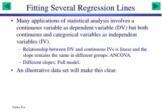
Fitting Several Regression Lines. Many applications of statistical analysis involves a continuous variable as dependent variable (DV) but both continuous and categorical variables as independent variables (IV).

Fitting Several Regression Lines
E N D
Presentation Transcript
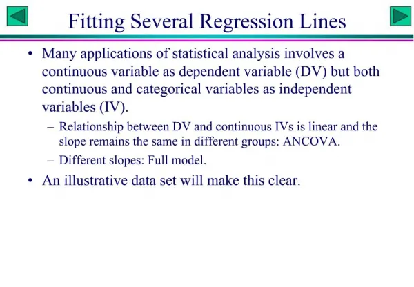
Fitting Several Regression Lines • Many applications of statistical analysis involves a continuous variable as dependent variable (DV) but both continuous and categorical variables as independent variables (IV). • Relationship between DV and continuous IVs is linear and the slope remains the same in different groups: ANCOVA. • Different slopes: Full model. • An illustrative data set will make this clear.
Fitting Several Regression Lines TM D MS A 1 11.5 A 2 13.8 A 3 14.4 A 4 16.8 A 5 18.7 B 1 10.8 B 2 12.3 B 3 13.7 B 4 14.2 B 5 16.6 C 1 13.1 C 2 16.2 C 3 19.0 C 4 22.9 C 5 26.5 • The muscle strength (MS) depends on the diameter of the muscle fiber and the type of muscle (TM). • Identify DV and IV. • How do we incorporate the qualitative variable in to the model? The dummy variables.
Two Scenarios Same intercept Different intercepts Different slopes: full model Same slope: ANCOVA
Two Scenarios Additive effect Multiplicative effect Same intercept Different intercepts Different slopes Same slope Y1 = a1 + b X Y2 = a2 + b X Y1 - Y2 = a1-a2 Y1 = a + b1 X Y2 = a + b2 X Y1 - Y2 = (b1-b2)X
Objectives • Obtain regression equations relating MS to D for each TM. • Compare the mean MS for the three TMs at a given level of D. Is it meaningful to compare the mean MS for the three TMs without specifying the level of D?
SAS Program Regression lines are fitted for all TMs simultaneously with the following statements: data Muscle; input TM $ D MS @@; cards; A 1 11.5 A 2 13.8 A 3 14.4 A 4 16.8 A 5 18.7 B 1 10.8 B 2 12.3 B 3 13.7 B 4 14.2 B 5 16.6 C 1 13.1 C 2 16.2 C 3 19.0 C 4 22.9 C 5 26.5 ; proc glm; class TM; model MS = TM|D / solution; run; proc sgplot; scatter x=D y=MS / group=TM; run;
Explaining the SAS Program The CLASS statement creates a dummy variable for each level of TM: DUMA = 1 if TM A = 0 otherwise DUMB = 1 if TM B = 0 otherwise DUMC = 0 MS = + A0DUMA + B0DUMB + 1D + A1DUMA*D + B1DUMB*D + The solution option prints estimates of the model coefficients.
SAS Output Dependent Variable: MS Sum of Mean TM DF Squares Square F Value Pr > F Model 5 258.727333 51.745467 263.71 0.0001 Error 9 1.766000 0.196222 Total 14 260.493333 R-Square C.V. Root MSE MS Mean 0.993221 2.762805 0.44297 16.0333 TM DF Type I SS Mean Square F Value Pr > F TM 2 98.001333 49.000667 249.72 0.0001 D 1 138.245333 138.245333 704.53 0.0001 D*TM 2 22.480667 11.240333 57.28 0.0001 TM DF Type III SS Mean Square F Value Pr > F TM 2 0.070242 0.035121 0.18 0.8390 D 1 138.245333 138.245333 704.53 0.0001 D*TM 2 22.480667 11.240333 57.28 0.0001
SAS Output T for H0: Pr > |T| Std Error of Parameter Estimate Parameter=0 Estimate INTERCEPT 9.490000000 B 20.43 0.0001 0.46459062 TM A 0.330000000 B 0.50 0.6275 0.65703036 B -0.020000000 B -0.03 0.9764 0.65703036 C 0.000000000 B . . . D 3.350000000 B 23.92 0.0001 0.14007934 D*TM A -1.610000000 B -8.13 0.0001 0.19810211 B -2.000000000 B -10.10 0.0001 0.19810211 C 0.000000000 B . . . • The fitted dummy variable model is • MS = 9.49 + 0.33 DUMA - 0.02 DUMB + 3.35 D - 1.61 DUMA*D - 2.00 DUMB*D
The Fitted Model • The fitted dummy variable model is • MS = 9.49 + 0.33 DUMA - 0.02 DUMB + 3.35 D - 1.61 DUMA*D - 2.00 DUMB*D • Equations for individual TMs are • A: MS = 9.49 + 0.33 + 3.35*D - 1.61*D = 9.82 + 1.74*D • B: MS = 9.49 - 0.02 + 3.35*D - 2.00*D = 9.47 + 1.35*D • C: MS = 9.49 - 0.00 + 3.35*D - 0.00*D = 9.49 + 3.35*D • This individual equations can be used for prediction (e.g., estimating mean MS for D=3.5 for TM=A).