A Coherence Function Statistic to Identify Coincident Bursts
A Coherence Function Statistic to Identify Coincident Bursts. Surjeet Rajendran, Caltech SURF Alan Weinstein, Caltech Burst UL WG, LSC meeting, 8/21/02. Cross-correlation of coincident burst data. After the search DSOs have identified data segments in which a burst is apparently present,

A Coherence Function Statistic to Identify Coincident Bursts
E N D
Presentation Transcript
A Coherence Function Statistic to Identify Coincident Bursts Surjeet Rajendran, Caltech SURF Alan Weinstein, Caltech Burst UL WG, LSC meeting, 8/21/02 AJW, Caltech, LIGO Project
Cross-correlation of coincident burst data • After the search DSOs have identified data segments in which a burst is apparently present, • And processing of the triggers identifies H2/L1 pairs which are coincident in time (to the level of resolution of the DSOs, eg, 1/8 second for tfclusters, ie, not as good as the required 10 msec), • And trigger level consistency cuts are made (overlapping frequency band, consistent amplitudes, etc) • We still may have to reduce the coincident fake rate. • SO, go back to the raw data and require consistency: • We seek a statistical measure which • reduces false coincidences significantly while • maintaining very high efficiency for even the faintest injected burst which triggers the DSOs • And can provide a better estimate of the start-time coincidence • We require this statistic to be robust even when • the two IFOs have very different sensitivities as well as • when there is a time delay of +/- 10 ms between the injected signals in the two IFOs. AJW, Caltech, LIGO Project
Cross-correlation statistic Let: X(t) = DT seconds of data from H2 Y(t) = DT seconds of data from L1. CXY(f) = Coherence function between X, Y. = abs(CSD(X, Y)2)/(PSD(X)*PSD(Y)) (CSD = Cross Spectral Density, PSD = Power Spectral density) Consider the statistic: CCS = Integral (CXY, {fmin, fmax}) (or) since we are sampling the data at discrete time intervals, we use the following discrete analog of (*): CCS = S CXY(f)*Df (between fmin and fmax) In our analysis, we use the value of DT = 1 second. The statistic will depend upon the value of DT and this dependence needs to be explored. AJW, Caltech, LIGO Project
Evaluation of the CCS • The idea behind this exercise is to determine the distribution of the CCS statistic before and after signal injection • and thereby hope to find a value of the CCS statistic which can then be used as a test to identify coincident bursts. • We would like this statistic to have a high efficiency of detection while maintaining a low fake rate. AJW, Caltech, LIGO Project
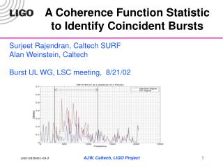
Determination of optimal values of fmin and fmax • We are considering ZM waveforms at a distance of 2 parsec (limit of sensitivity during E7) • To find the optimal range of values of fmin and fmax, we plot CXY(f) for the case when there are no injected burst signals in H2, L1 and compare it with the case when we inject signals. AJW, Caltech, LIGO Project
CCS for different ZM waveforms AJW, Caltech, LIGO Project
Limits of integration • From the above plots, it is clear that the region of interest lies between ~250 Hz – 1000 Hz. • This is consistent with the fact that ZM supernovae have little power beyond 1000 Hz and the fact that LIGO has its peak sensitivity in this region. • The plots also indicate that the CCS statistic would be of little use in detecting some weak waveforms (eg: A1B1G5). • Details: • The raw E7 data has been whitened and resampled to 4096 Hz • The injected signals have been filtered through the calibrated transfer function (strain LSC-AS_Q counts), then whitened and resampled like the data. • So far, we have been using 300-1000 Hz as our limits of integration. AJW, Caltech, LIGO Project
Procedure for evaluating CCS • We take N (N = 360 in our case) seconds of data from L1 and H2. • We break the N second dataset into (N/DT) intervals of length DT each (DT= 1 second in our case). • We then estimate the distribution of the CCS statistic on the raw data by forming (N/ DT)2 coincidences between them and computing the CCS statistic between the DT second intervals thus generated. • We histogram the results to arrive at the distribution of the CCS statistic on the raw data. • Since the CCS statistic test will be used only on the data sections that trigger the DSOs, we perform the same analysis on the data sections between the times t and t + DT where t corresponds to the time identified by the DSO as the start time of the burst which triggered the DSO. • We then inject ZM waveform signals in the (N/DT) intervals of length DT. • The distribution of the CCS statistic after signal injection is similarly studied. • We then inject the ZM waveform signals with a time delay of 10 ms (H2/L1 light travel time) between them and estimate the CCS statistic by the above method. AJW, Caltech, LIGO Project
Summary of results AJW, Caltech, LIGO Project
Observations • the distribution of the CCS statistic on the data sections identified by the DSOs as containing bursts is very similar to the distribution of the CCS statistic on random DT seconds of data from L1 and H2. • The peak of the CCS statistic distribution when the signal between H2, L1 is delayed by 10 ms is occurs at a slightly lower bin than the peak of the distribution when there is no delay. • However, we can still produce an efficient value of the CCS statistic which maintains high rates of efficiency while minimizing the fake rate. AJW, Caltech, LIGO Project
Cut on CCS. Efficiency vs fake rate reduction AJW, Caltech, LIGO Project
Some things to be done • Estimate the CCS between 250-1000 Hz. We expect the results to be better than the results obtained above (using 300-1000 Hz). • Explore the dependence of the CCS on DT. Can we estimate DT to 10 msec or better? • Explore other waveforms • S1 data • Automate, using LDAS (or DMT). AJW, Caltech, LIGO Project