Download

1 / 15
150 likes | 438 Vues
Cass Apollo Petrus ( petrus@csit.fsu.edu ) Florida Atlantic University Honors College, Jupiter, Florida 33458 and Dr. Ali Uzun (uzun@csit.fsu.edu) School of Computational Science and Information Technology, Florida State University, Tallahassee, Florida 32306-4120.

E N D
Cass Apollo Petrus (petrus@csit.fsu.edu) Florida Atlantic University Honors College, Jupiter, Florida 33458 and Dr. Ali Uzun (uzun@csit.fsu.edu) School of Computational Science and Information Technology, Florida State University, Tallahassee, Florida 32306-4120 NUMERICAL INVESTIGATIONS OF FINITE DIFFERENCE SCHEMES
Abstract This paper presents some of the differences between using different high-order compact schemes compared to explicit finite differences for Computational Aeroacoustics (CAA). By testing on the Linearised Euler Equations (LEE), we have a benchmark test for these methods. In general, the higher order compact schemes performed better then the explicit finite difference equations.
Introduction Computational Aeroacoustics is a field born from public concern over noise emissions from both fixed and rotary wing aircraft. Essentially, this discipline is devoted to the accurate prediction of sound from aircraft nose-cones, fuselages, wings, and engines. The main difficulties, however, are posed by the fact that prediction of the small amplitude acoustic fluctuations and propagation because these models require high accuracy, usually at the expense of computational power. Koutsavdis et al. point out that over the past few years, new schemes have arisen that are up for the challenge, offering more accuracy with less demand of processing power. The schemes that catch our attention are those of S.K. Lele, who presented a family of compact schemes.
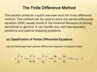
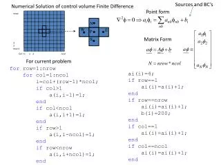
We combine this with the following boundary conditions Methods To model the Linearised Euler Equation in one dimension, we compute the derivatives and integrals numerically with Fortran 77. The one-dimensional LEE equations are:
where 2. An explicit fourth order scheme 4. An implicit sixth order scheme We use the following schemes: 1. An explicit second order scheme 3. An implicit fourth order scheme (Pad scheme)
Methods cont. Computations involving the explicit schemes are fairly straight forward, but because of their lower order, they provide less accuracy. The implicit scheme, while providing more accuracy, requires some matrix solving, which takes more processing power. Luckily, the types of matrices generated by equations like the one above have a form easily solved with algorithms; this makes them much more practical to solve than a normal n x n matrix. To solve the LEE, we must first apply the initial condition; then, we obtain derivatives of the , p, and u values with respect to the spatial variable x for all values on the wave pulse. We integrate using the standard fourth order Runge-Kutta time advancement scheme as suggested by Koutsavdis et.al.
Results To analyse the effectiveness of the different schemes, we examine how the graphs compare to the analytical solutionas well as compute the root mean square (RMS) of the analytical and numerical solutions. We present a table of the RMS values and graphs of the data at 62, 125, and 187 grid points which correspond to 5, 10, and 15 points on the wave pulse respectively.
The overall conclusion is that the higher order compact schemes perform better compared to the explicit schemes (see table 1). For the lowest order scheme, we find very little accuracy even with 15 points on the pulse. Due to the low order, phase error shows up in the approximation. As expected, for each of the schemes, increased number of grid points increases its resemblance to the analytical solution Conclusion
[1] Koutasavdis, E.K.; Blaisdell, G.A.; Lyrintzis, A.S.; “On the Use of Compact Schemes with Spatial Filtering in Computational Aeroacoustics,” American Institute of Aeronautics & Astronautics. AIAA 99-0360, pp. 1-14 [2] Lele, S.K., “Compact Finite Difference Schemes with Spectral-like Resolution,”Journal of Computational Physics, Vol. 103, 1992, pp. 16-42 [3] Hoffmann, Klaus A.; Chiang, Steve T.; Computational Fluid Dynamics Vol. 3. 2000. pp.117-138. References
Appendix: Figures Graph 2-2nd order with 10 points Graph 1-2nd order with 5 points Graph 3-2nd order with 15 points Graph 4-4th order explicit with 5 points
Graph 5 - 4th order explicit with 10 points Graph 6 - 4th order explicit with 15 points
Graph 8 - 4th order implicit with 10 points Graph 7 - 4th order implicit with 5 points
Graph 9 - 4th order implicit with 15 points Graph 10 - 6th order implicit with 5 points
Graph 11 - 6th order implicit with 10 points Graph 12 - 6th order implicit with 15 points