HW/SW Synthesis
430 likes | 852 Vues
HW/SW Synthesis. Outline. Synthesis CFSM Optimization Software synthesis Problem Task synthesis Performance analysis Task scheduling Compilation. POLIS Methodology. Graphical EFSM+ Esterel. Java. EC. Compilers. SW Synthesis. HW Synthesis. CFSMs. Partitioning. SW Estimation.

HW/SW Synthesis
E N D
Presentation Transcript
Outline • Synthesis • CFSM Optimization • Software synthesis • Problem • Task synthesis • Performance analysis • Task scheduling • Compilation
POLIS Methodology ................ Graphical EFSM+ Esterel Java EC Compilers SW Synthesis HW Synthesis CFSMs Partitioning SW Estimation HW Estimation Logic Netlist HW/SW Co-Simulation Performance/trade-off Evaluation Formal Verification SW Code + RTOS • Aptix Board Consists of • micro of choice • FPGA’s • FPIC’s Physical Prototyping
Hardware - Software Architecture • Hardware: • Currently: • Programmable processors (micro-controllers, DSPs) • ASICs (FPGAs) • Software: • Set of concurrent tasks • Customized Real-Time Operating System • Interfaces: • Hardware modules • Software procedures (polling, interrupt handlers, ...)
System Partitioning Scheduler e2 CFSM1 CFSM4 port1 e2 e5 port7 port5 e3 CFSM2 e7 port2 CFSM5 e1 CFSM6 e3 HW partition 1 e9 port6 port3 e9 e8 CFSM7 SW partition 3 CFSM3 HW partition2
Software Synthesis • Two-level process • “Technology” (processor) independent: • best decision/assignment sequence given CFSM • “Technology” (processor) dependent: • conversion into machine code • instruction selection • instruction scheduling • register assignment (currently left to compiler) • need performance and cost analysis • Worst Case Execution Time • code and data size
Software Synthesis • Technology-independent phase: • Construction of Control-Data Flow Graph from CFSM (based on BDD representation of Transition Function) • Optimization of CDFG for • execution speed • code size (based on BDD sifting algorithm) • Technology-dependent phase: • Creation of (restricted) C code • Cost and performance analysis • Compilation
Software Implementation Problem • Input: • Set of tasks (specified by CFSMs) • Set of timing constraints (e.g., input event rates and response constraints) • Output: • Set of procedures that implement the tasks • Scheduler that satisfies the timing constraints • Minimizing: • CPU cost • Memory size • Power, etc.
Software Implementation • How to do it ? • Traditional approach: • Hand-coding of procedures • Hand-estimation of timing input to scheduling algorithms • Long and error-prone • Our approach: three-step automated procedure: • Synthesize each task separately • Extract (estimated) timing • Schedule the tasks • Customized RT-OS (scheduler + drivers)
Software Implementation • Current strategy: • Iterate between synthesis, estimation and scheduling • Designer chooses the scheduling algorithm • Future work: • Top-down propagation of timing constraints • Software synthesis under constraints • Automated scheduling selection (based on CPU utilization estimates)
Software Synthesis Procedure Specification, partitioning Code generation S-graph synthesis Compilation fail Timing estimation Testing, validation pass not feasible Production Scheduling, validation feasible
Task Implementation • Goal: quick response time, within timing and size constraints • Problem statement: • Given a CFSM transition function and constraints • Find a procedure implementing the transition function while meeting the constraints • The procedure code is acyclic: • Powerful optimization and analysis techniques • Looping, state storage etc. are implemented outside (in the OS)
SW Modeling Issues • The software model should be: • Low-level enough to allow detailed optimization and estimation • High-level enough to avoid excessive details e.g. register allocation, instruction selection • Main types of “user-mode” instructions: • Data movement • ALU • Conditional/unconditional branches • Subroutine calls • RTOS handles I/O, interrupts and so on
SW Modeling Issues • Focus on control-dominated applications • Address only CFSM control structure optimization • Data path left as “don’t touch” • Use Decision Diagrams (Bryant ‘86) • Appropriate for control-dominated tasks • Well-developed set of optimization techniques • Augmented with arithmetic and Boolean operators, to perform data computations
ROBDDs • Reduced Ordered BDDs[Bryant 86] • A node represents a function given by the Shannon decomposition • f = x f x + x f x • Variable appears onceon any path from root to terminal • Variables are ordered • No two vertices represent the same function • Canonical • Two functions are equal if and only if their • BDDs are isomorphic Þ direct application in equivalence checking f = x1 + x2 x3 f x1 x1 1 0 x2 1 0 f x3 x1 0 1 0 1 ROBDD
ROBDDs and Combinational Verification • Given two circuits: • Build the ROBDDs of the outputs in terms of the primary inputs • Two circuits are equivalent if and only if the ROBDDs are isomorphic • Complexity of verification depends on the sizeof ROBDDs • Compact in many cases
ROBDDs and Memory Explosion • ROBDDs are not always compact • Size of an ROBDD can be exponential in number of variables • Can happen for real life circuits also • e.g. Multipliers • Commonly known as: • Memory Explosion Problem of ROBDDs
Technique for Handling ROBDD Memory Explosion Enhancements Variable Ordering ROBDDs Node Decomp. Relax Ordering Partitioning OFDDs, OKFDDs Partitioned ROBDDs Free BDDs All the representations are canonical Þ combinational equivalence checking
0 1 Handling Memory Explosion: Variable Ordering • BDD size very sensitive to variable ordering a1b1 + a2b2 + a3b3 a1 a1 a2 a2 b1 a2 a3 a3 a3 a3 b1 b1 b1 b1 b2 a3 b2 b2 b3 b3 0 1 1 0 Good Ordering: 8 nodes Bad Ordering: 16 nodes
a2 b1 b1 b2 0 1 Handling Memory Explosion: Variable Ordering • Good static as well as dynamic ordering techniques exist • Dynamic variable reordering [Rudell 93] • Change variable order automatically during computations • Repeatedly swap a variable with adjacent variable • Swapping can be done locally • Select the best location a1b1 + a2b2 a1 a1 0 1 0 1 a2 b1 a2 b2 0 1
SW Model: S-graphs • Acyclic extended decision diagram computing a transition function • S-graph structure: • Directed acyclic graph • Set of finite-valued variables • TEST nodes evaluate an expression and branch accordingly • ASSIGN nodes evaluate an expression and assign its result to a variable • Basic block + branch is a general CDFG model (but we constrain it to be acyclic for optimization)
BEGIN a := 0 a := a + 1 END An Example of S-graph detect(c) • input event c • output event y • state int a • input int b • forever • if (detect(c)) • if (a < b) • a := a + 1 • emit(y) • else • a := 0 • emit(y) a<b T T F F emit(y)
S-graphs and Functions • Execution of an s-graph computes a function from a set of input and state variables to a set of output and state variables: • Output variables are initially undefined • Traverse the s-graph from BEGIN to END • Well-formed s-graph: • Every time a function depending on a variable is evaluated, that variable has a defined value • How do we derive an s-graph implementing a given function ?
S-graphs and Functions • Problem statement: • Given: a finite-valued multi-output function over a set of finite-valued variables • Find: an s-graph implementing it • Procedure based on Shannon expansion f = x fx + x’ fx’ • Result heavily depends on ordering of variables in expansion • Inputs before outputs: TESTs dominate over ASSIGNs • Outputs before inputs: ASSIGNs dominate over TESTs
Example of S-graph Construction x = a b + c y = a b + d a 0 1 Order: a, b, c, d, x, y (inputs before outputs) b 0 c 1 0 1 0 d 1 0 d 1 x := 0 x := 0 x := 1 x := 1 y := 0 y := 1 y := 0 y := 1
Example of S-graph Construction x = a b + c y = a b + d a 0 1 Order: a, b, x, y, c, d (interleaving inputs and outputs) b 0 1 x := c x := 1 y := d y := 1
S-graph Optimization • General trade-off: • TEST-based is faster than ASSIGN-based (each variable is visited at most once) • ASSIGN-based is smaller than TEST-based (there is more potential for sharing) • Implemented as constrained sifting of the Transition Function BDD • The procedure can be iterated over s-graph fragments: • Local optimization, depending on fragment criticality (speed versus size) • Constraint-driven optimization (still to be explored)
From S-graphs to Instructions • TEST nodes conditional branches • ASSIGN nodes ALU ops and data moves • No loops in a single CFSM transition • (User loops handled at the RTOS level) • Data flow handling: • “Don’t touch” them (except common sub-expression extraction) • Map expression DAGs to C expressions • C compiler allocates registers and select op-codes • Need source-level debugging environment (with any of the chosen entry languages)
Software Synthesis Procedure Specification, partitioning Code generation S-graph synthesis Compilation fail Timing estimation Testing, validation pass not feasible Production Scheduling, validation feasible
Problems in Software Performance Estimation How to link behavior to assembly code?-> Model C code generated from S-graph and use a set of cost parameters How to handle the variety of compilers and CPUs?
Execution Time of a Path and the Code Size Property : Form of each statement is determined by type of corresponding node. T = ƒ°pi Ct( (i), (i)) node_type_of variable_type_of struct pi: takes value 1 if node i is on a path, otherwise 0. Ct(n,v): execution time for node type n and variable type v. S = ƒ°Cs( (i), (i)) node_type_of variable_type_of struct Cs(n,v): code size for node type n and variable type v.
Cost Parameters * Pre-calculated cost parameters for: (1) Ct(n,v), Cs(n,v): Execution time and code size for node type n and variable type v. (2) Tpp, Spp: Pre- and post- execution time and code size. (3) Tinit, Sinit: Execution time and code size for local variable initialization.
Problems in Software Performance Estimation How to link behavior to assembly code? How to handle the variety of compilers and CPUs?-> prepare cost parameters for each target
Algorithm • Preprocess: extracting set of cost parameters. • Weighting nodes and edges in given S-graph with cost parameters. • Traversing weighted S-graph. • Finding maximum cost path and minimum cost path using Depth-First Search on S-graph. • Accumulating 'size' costs on all nodes.
S-graph Level Estimation :Algorithm Cost C is a triple (min_time, max_time, code_size) Algorithm: SGtrace (sgi) if (sgi == NULL) return (C(0, ,0)); if (sgi has been visited) return ( pre-calculated Ci(*,*,0) associated with sgi ); Ci = initialize (max_time = 0, min_time = , code_size = 0); for each child sgj of sgi { Cij = SGtrace (sgj) + edge cost for edge eij; Ci.max_time = max(Ci.max_time, Cij.max_time); Ci.min_time = min(Ci.min_time, Cij.min_time); Ci.code_size += Cij.code_size; } Ci += node cost for node sgi; return (Ci);
Experiments * Proposed methods implemented and examined in POLIS system. * Target CPU and compiler: M68HC11 and Introl C compiler. * Difference D is defined as
Performance and Cost Estimation: Summary • S-graph: low-level enough to allow accurate performance estimation • Cost parameters assigned to each node, depending on: • System type (CPU, memory, bus, ...) • Node and expression type • Cost parameters evaluated via simple benchmarks • Need timing and size measurements for each target system • Currently implemented for MIPS, 68332 and 68HC11 processors
BEGIN a := 0 a := a + 1 END Performance and Cost Estimation • Example: 68HC11 timing estimation • Cost assigned to s-graph edges (Different for taken/not taken branches) • Estimated time: • Min: 26 cycles • Max: 126 cycles • Accuracy: within 20% of profiling 40 a<b detect(c) T 41 63 26 T F F 18 9 emit(y) 14
Open Problems • Better synthesis techniques • Add state variables to simplify s-graph • Performance-driven synthesis of critical paths • Exact memory/speed trade-off • Estimation of caching and pipelining effects • May have little impact on control-dominated systems (frequent branches and context switches) • Relatively easy during co-simulation