Download
1 / 28
340 likes | 757 Vues
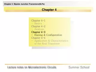
Chapter3:Bipolar Junction Transistors (BJTs). 1. Figure 3.1 A simplified structure of the npn transistor. Figure 3.2 A simplified structure of the pnp transistor.

E N D
Figure 3.1 A simplified structure of the npn transistor. Figure 3.2 A simplified structure of the pnp transistor.
Figure 3.3 Current flow in an npn transistor biased to operate in the active mode. (Reverse current components due to drift of thermally generated minority carriers are not shown.) Figure 5.6 Cross-section of an npn BJT.
Figure 3.4 Profiles of minority-carrier concentrations in the base and in the emitter of an npn transistor operating in the active mode: vBE > 0 and vCB ³ 0.
Figure 3.5 Large-signal equivalent-circuit models of the npn BJT operating in the forward active mode.
Figure 3.9 The iC–vCB characteristic of an npn transistor fed with a constant emitter current IE. The transistor enters the saturation mode of operation for vCB < –0.4 V, and the collector current diminishes.
Figure 3.11 Large-signal model for the pnp transistor operating in the active mode. Figure 3.12 Circuit symbols for BJTs.
Figure 3.13 Voltage polarities and current flow in transistors biased in the active mode. Example:β=100, VBE=0.7v at Ic=1mA For Ic=2mA and Vc= 5v, what are the different values of Rc=?, VBE=? IE=?, RE=? Figure 3.14 Circuit for Example 5.1.
Application 1: • In the circuit shown below (Fig E3.15), the voltage at the emitter was measured and found to be -0.7v. If β=50, find IE?, IC?, IB?, VC? Figure E3.15
Application 1: P 423 Figure 5.34 Analysis of the circuit for Example 5.4: (a) circuit; (b) circuit redrawn to remind the reader of the convention used in this book to show connections to the power supply
Application 2: P 422 Figure 5.35 Analysis of the circuit for Example 5.5. Note that the circled numbers indicate the order of the analysis steps.
Application 3: Determine the voltage at all nodes and the current through all branches Figure 5.37 Example 5.7: (a) circuit
Application 4: Figure 5.38 Example 5.8: (a) circuit; (b) analysis with the steps indicated by the circled numbers.
Application 5: For the emitter bias network determine a. lB b. IC c. VCE d. VC e. VE f. VB g. VBC Figure 5.39 Example 5.9: (a) circuit; (b) analysis with steps numbered.
Application 5: Figure 5.40 Circuits for Example 5.10.
Transistor Switch A transistor when used as a switch is simply being biased so that it is in cutoff (switched off) or saturation (switched on). Remember that the VCE in cutoff is VCC and 0 V in saturation. VCE(cutoff) = VCC IC(sat) = (VCC – VCE(sat))/βDC IB(min) = Ic(sat)/βDC
Biasing in BJT Amplifier circuits Figure 5.44 (P 437) Classical biasing for BJTs using a single power supply: (a) circuit; (b) circuit with the voltage divider supplying the base replaced with its Thévenin equivalent.
The collector current and transductance Figure 5.48 (a) Conceptual circuit to illustrate the operation of the transistor as an amplifier. (b) The circuit of (a) with the signal source vbe eliminated for dc (bias) analysis.
The hybrid π model Figure 5.50( P 448) The amplifier circuit of Fig. 5.48(a) with the dc sources (VBE and VCC) eliminated (short circuited). Thus only the signal components are present. Note that this is a representation of the signal operation of the BJT and not an actual amplifier circuit. Figure 5.51 Two slightly different versions of the simplified hybrid-p model for the small-signal operation of the BJT. The equivalent circuit in (a) represents the BJT as a voltage-controlled current source (a transconductance amplifier), and that in (b) represents the BJT as a current-controlled current source (a current amplifier).
Application of the small-signal equivalent circuits Figure 5.53 Example 5.14: (a) circuit; (b) dc analysis; (c) small-signal model.
Performing small-signal analysis directly on the circuit diagram Figure 5.58 The hybrid-p small-signal model, in its two versions, with the resistance ro included.
Figure 5.59 Basic structure of the circuit used to realize single-stage, discrete-circuit BJT amplifier configurations.
Common Emitter Input resistance moderate/small Output resistance large Open Circuit Voltage gain large Short Circuit Current gain large Figure 5.60(a) A common-emitter amplifier using the structure of Fig. 5.59. (b) Equivalent circuit obtained by replacing the transistor with its hybrid-p model. Large voltage and current gain but Rin and Ro not good for voltage amplifier.
Common Emitter with RE Re increases Rin but reduces open circuit voltage gain. Current gain and output resistance are unchanged. Input resistance Open Circuit Voltage gain reduced increased Voltage gain reduced by ~ (1+gmRe); Rib increased by this factor. Rib greatly increased by resistance reflection rule (Miller) Figure 5.61 (a) A common-emitter amplifier with an emitter resistance Re. (b) Equivalent circuit obtained by replacing the transistor with its T model.
Common Base Input resistance Open Circuit Voltage gain Short Circuit Current gain small large unity Output resistance Non-inverting version of common emitter. large Good for unity gain current buffer. Figure 5.62 (a) A common-base amplifier using the structure of Fig. 5.59. (b) Equivalent circuit obtained by replacing the transistor with its T model.
Common Collector Figure 5.63 (a) An emitter-follower circuit based on the structure of Fig. 5.59. (b) Small-signal equivalent circuit of the emitter follower with the transistor replaced by its T model augmented with ro. (c) The circuit in (b) redrawn to emphasize that ro is in parallel with RL. This simplifies the analysis considerably.
Input resistance large Output resistance small Open Circuit Voltage gain Current gain ~unity large Voltage gain ~1 so emitter follows base input voltage (emitter follower) Good for amplifier output stage: large Rin, small Rout.
Figure 5.71 (a) Capacitively coupled common-emitter amplifier. (b) Sketch of the magnitude of the gain of the CE amplifier versus frequency. The graph delineates the three frequency bands relevant to frequency-response determination.