Smoothing bathymetry tutorial
Smoothing bathymetry tutorial. Ivica Janekovic & Mathieu Dutour Sikiric* ivica@soest.hawaii.edu * IRB. Intro. Terrenian following coordinate system (sigma coordinate - Philliips 1957) Problem of derivation @ z df/dx|z=df/dx|s+dh/dx*df/ds Introduction of error in HPG calcs

Smoothing bathymetry tutorial
E N D
Presentation Transcript
Smoothing bathymetrytutorial Ivica Janekovic & Mathieu Dutour Sikiric* ivica@soest.hawaii.edu * IRB
Intro • Terrenian following coordinate system (sigma coordinate - Philliips 1957) • Problem of derivation @ z df/dx|z=df/dx|s+dh/dx*df/ds • Introduction of error in HPG calcs • Smagorinsky 1967,Janjic 1997, Haney 1991,… • Realistic / numerically stabile (HPGE free) • Definition of rx0(h), rx1 is more complicated • Filtering (Shapiro, Laplacian, simple convolution…) • Mellor ‘94 (volume conservative) • Martinho – Betteen 2006 (increase bathy) • LP technique with variable rx0,… • Alternatives ?
ROMS vertical This routine sets and initializes relevant variables associated with the vertical terrain-following coordinates transformation. Definitions: N(ng) : Number of vertical levels for each nested grid. zeta : time-varying free-surface, zeta(x,y,t), (m) h : bathymetry, h(x,y), (m, positive, maybe time-varying) hc : critical (thermocline, pycnocline) depth (m, positive) z : vertical depths, z(x,y,s,t), meters, negative z_w(x,y,0:N(ng)) at W-points (top/bottom cell) z_r(z,y,1:N(ng)) at RHO-points (cell center) z_w(x,y,0 ) = -h(x,y) z_w(x,y,N(ng)) = zeta(x,y,t) s : nondimensional stretched vertical coordinate, -1 <= s <= 0 s = 0 at the free-surface, z(x,y, 0,t) = zeta(x,y,t) s = -1 at the bottom, z(x,y,-1,t) = - h(x,y,t) sc_w(k) = (k-N(ng))/N(ng) k=0:N, W-points sc_r(k) = (k-N(ng)-0.5)/N(ng) k=1:N, RHO-points C : nondimensional vertical stretching function, C(s), -1 <= C(s) <= 0 C(s) = 0 for s = 0, at the free-surface C(s) = -1 for s = -1, at the bottom Cs_w(k) = F(s,theta_s,theta_b) k=0:N, W-points Cs_r(k) = C(s,theta_s,theta_b) k=1:N, RHO-points Zo : vertical transformation functional, Zo(x,y,s): Zo(x,y,s) = H(x,y)C(s) separable functions Two vertical transformations are supported, z => z(x,y,s,t): (1) Original transformation (Shchepetkin and McWilliams, 2005): In ROMS since 1999 (version 1.8): z(x,y,s,t) = Zo(x,y,s) + zeta(x,y,t) * [1 + Zo(x,y,s)/h(x,y)] where Zo(x,y,s) = hc * s + [h(x,y) - hc] * C(s) Zo(x,y,s) = 0 for s = 0, C(s) = 0, at the surface Zo(x,y,s) = -h(x,y) for s = -1, C(s) = -1, at the bottom (2) New transformation: In UCLA-ROMS since 2005: z(x,y,s,t) = zeta(x,y,t) + [zeta(x,y,t) + h(x,y)] * Zo(x,y,s) where Zo(x,y,s) = [hc * s(k) + h(x,y) * C(k)] / [hc + h(x,y)] Zo(x,y,s) = 0 for s = 0, C(s) = 0, at the surface Zo(x,y,s) = -1 for s = -1, C(s) = -1, at the bottom At the rest state, corresponding to zero free-surface, this transformation yields the following unperturbed depths, zhat: zhat = z(x,y,s,0) = h(x,y) * Zo(x,y,s) = h(x,y) * [hc * s(k) + h(x,y) * C(k)] / [hc + h(x,y)] and d(zhat) = ds * h(x,y) * hc / [hc + h(x,y)] As a consequence, the uppermost grid box retains very little dependency from bathymetry in the areas where hc << h(x,y), that is deep areas. For example, if hc=250 m, and h(x,y) changes from 2000 to 6000 meters, the uppermost grid box changes only by a factor of 1.08 (less than 10%). Notice that: * Regardless of the design of C(s), transformation (2) behaves like equally-spaced sigma-coordinates in shallow areas, where h(x,y) << hc. This is advantageous because high vertical resolution and associated CFL limitation is avoided in these areas. * Near-surface refinement is close to geopotential coordinates in deep areas (level thickness do not depend or weakly-depend on the bathymetry). Contrarily, near-bottom refinement is like sigma-coordinates with thicknesses roughly proportional to depth reducing high r-factors in these areas. • ./ROMS/Utility/set_scoord.F
ROMS vertical ELSE IF (Vtransform(ng).eq.2) THEN DO j=JstrR,JendR DO i=IstrR,IendR # if defined SEDIMENT && defined SED_MORPH h(i,j)=h(i,j)-bed_thick(i,j,nstp)+bed_thick(i,j,nnew) # endif # if defined WET_DRY IF (h(i,j).eq.0.0_r8) THEN h(i,j)=eps END IF # endif z_w(i,j,0)=-h(i,j) END DO DO k=1,N(ng) cff_r=hc(ng)*SCALARS(ng)%sc_r(k) cff_w=hc(ng)*SCALARS(ng)%sc_w(k) cff1_r=SCALARS(ng)%Cs_r(k) cff1_w=SCALARS(ng)%Cs_w(k) DO i=IstrR,IendR hwater=h(i,j) # ifdef ICESHELF hwater=hwater-ABS(zice(i,j)) # endif hinv=1.0_r8/(hc(ng)+hwater) cff2_r=(cff_r+cff1_r*hwater)*hinv cff2_w=(cff_w+cff1_w*hwater)*hinv z_w(i,j,k)=Zt_avg1(i,j)+(Zt_avg1(i,j)+hwater)*cff2_w z_r(i,j,k)=Zt_avg1(i,j)+(Zt_avg1(i,j)+hwater)*cff2_r # ifdef ICESHELF z_w(i,j,k)=z_w(i,j,k)-ABS(zice(i,j)) z_r(i,j,k)=z_r(i,j,k)-ABS(zice(i,j)) # endif Hz(i,j,k)=z_w(i,j,k)-z_w(i,j,k-1) END DO END DO END DO END IF • ./ROMS/Nonlinear/set_depth.F ----------------------------------------------------------------------- Original formulation: Compute vertical depths (meters, negative) at RHO- and W-points, and vertical grid thicknesses. Various stretching functions are possible. z_w(x,y,s,t) = Zo_w + zeta(x,y,t) * [1.0 + Zo_w / h(x,y)] Zo_w = hc * [s(k) - C(k)] + C(k) * h(x,y) ----------------------------------------------------------------------- ----------------------------------------------------------------------- New formulation: Compute vertical depths (meters, negative) at RHO- and W-points, and vertical grid thicknesses. Various stretching functions are possible. z_w(x,y,s,t) = zeta(x,y,t) + [zeta(x,y,t)+ h(x,y)] * Zo_w Zo_w = [hc * s(k) + C(k) * h(x,y)] / [hc + h(x,y)] -----------------------------------------------------------------------
Goal • to have as less as possible rx0; rx1 but to keep basin realistic as possible at the same time ;) • in ROMS we can use different set of params: • theta_s, theta_b, hc, vtransformation, vstretching, N • different domains different rx0,rx1 • user should spend some initial time to set it up properly -> one time investment • run HPGE calc to see what’s happening inside domain • some tools available (matlab, but could be transfered) Example …
Example • web based utility at ROMS host http://nelson.soest.hawaii.edu:8080/~ivica/SMOOTH_BATHYMETY/ • for testing only, limits of PC • prepare hraw & mask and save it in .mat • upload that file and choose the roms params • be careful what you get • 2 stage reduce rx0 first (different options) and than rx1 • output: bathy_rx0_done: [35x59 double] rx1matrix_after_rx1: [35x59 double] bathy_rx0_rx1_done: [35x59 double] rx1matrix_after_rx0: [35x59 double]
additional tools • smooth with additional constraints • define max. amplitude of change [m x n] • define sign of change [m x n] • define target rx0_v [m x n] • we can afford bigger rx0 at shallow regions, so keep real bathy as possible • reduce more rx0 (smooth more) in deeper parts where HPGE is growing • rx0_max=0.25; rx0_v=rx0_max*(1-test.h/max(test.h(:)));[m x n] • rx0_v(find(rx0_v<0.05))=0.05; • use “positive”, “negative”, play with mask, H(mask)
test case for HIOG -> variables hraw & mask (check min depht, no nans) [50 x 124]
output from smoothing only rx0 is not good enough >> new_bathy = vertical: [1x1 struct] rx1_and_rx0_optimized: [50x124 double] rx0_optimized: [50x124 double] >> new_bathy.vertical ans = ThetaS: 7 ThetaB: 0.1 N: 30 Vtransform: 2 Vstretching: 2 hc: 100 >> tmp.h=new_bathy.rx0_optimized; >> rx1=rx1_matrix(tmp);max(rx1(:)) ans = 10.369 >> tmp.h=new_bathy.rx1_and_rx0_optimized; >> rx1=rx1_matrix(tmp);max(rx1(:)) ans = 4